
This post begins a multi-part exploration of the role of constraints in mechanical systems. It builds on the general framework discussed in the last post but does so by examining specific examples. This month the focus will be on the simplest example of a constraint: a bead sliding on a wire.
Despite its trivial appearance, this problem is surprisingly complex due to the presence of the constraint and, as will be shown below, provides significant obstacles to obtaining an accurate numerical solution.
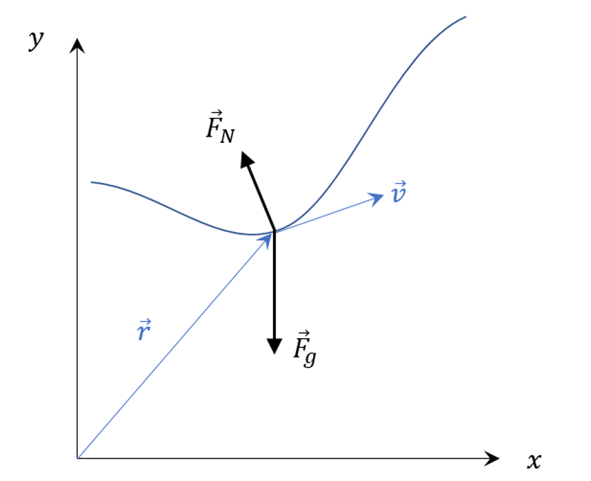
The following figure shows a portion of the wire, the position, $$\vec r$$, and the velocity, $$\vec v$$, of the bead, and the two forces acting upon it; namely the force of gravity $${\vec F}_g$$ and the normal force $${\vec F}_N$$. With this information, it is, in principle, easy to solve for the motion of the bead via Newton’s laws. There are several equivalent ways of carrying this out but I’ll be focusing on the most geometric of these.
The position of a particle in a plane is given by
\[ \vec r = \left[ \begin{array}{c} x \\ y \end{array} \right] \; . \]
Since the bead must remain on the wire, only those values of $$y$$ satisfying $$y = f(x)$$ are permissible and the position can now be written as
\[ \vec r = \left[ \begin{array}{c} x \\ f(x) \end{array} \right ] \; . \]
The velocity is then given by
\[ \vec v = \left[ \begin{array}{c} 1 \\ f'(x) \end{array} \right] \dot x \; .\]
The normal to the curve, $$\hat N$$, is obtained from the requirement that motion consistent with the constraint must always be perpendicular to the normal to the wire at the point in question:
\[ \hat N \cdot d\vec r = N_x dx + N_y dy = 0 \;.\]
Using the constraint equation $$y – f(x) = 0$$ and then taking the differential yields the component form
\[ dy – f'(x) dx = 0 \; , \]
from which it is easy to read off the components of the normal (the sign being chosen so that $$\vec F_N$$ is in opposition $$\vec F_g$$. Subsequent normalization gives
\[ \hat N = \frac{1}{\sqrt{1+f’^2}} \left[ \begin{array}{c} -f'(x) \\ 1 \end{array} \right] \; .\]
The forces on the bead are due to gravity
\[ \vec F_g = – m g \hat y \]
and the normal force
\[ \vec F_N = -(\vec F_g \cdot \hat N) \hat N = \frac{m g}{1+f’^2} \left[ \begin{array}{c} -f’ \\ 1 \end{array} \right]\; \]
For notational convenience in what follows, define
\[ \tau = \frac{1}{1+f’2} \; .\]
Summing the forces and inserting them into Newton’s second law leads to the following equations (eliminating $$m$$ from both sides)
\[ \left[ \begin{array}{c} \ddot x \\ \ddot y \end{array} \right] = \left[ \begin{array}{c} -g \tau f’ \\ g (\tau -1 ) \end{array} \right] = \left[ \begin{array}{c} -g \tau f’ \\ – g \tau f’^2 \end{array} \right] \; .\]
Expressing Newton’s equations in state-space form then yields
\[ \frac{d}{dt} \left[ \begin{array}{c} x \\ y\\ \dot x \\ \dot y \end{array} \right] = \left[ \begin{array}{c} \dot x \\ \dot y \\ – g \tau f’ \\ – g \tau f’^2 \end{array} \right] \; .\]
These equations are easy to code and couple to a standard solver. I chose to implement this system in Python and SciPy as follows:
def roller_coaster(state,t,geometry,g):
    #unpack the state
    x     = state[0]
    y     = state[1]
    vx    = state[2]
    vy    = state[3]

    #evaluate the geometry
    f,df,df2 = geometry(x)
    tau      = 1.0/(1.0+df**2)

    #return the derivative
    return np.array([vx,vy,-g*tau*df,-g*tau*df**2])
where the function geometry can be any curve in the $$x-y$$ plane. For example, for a bead sliding down a parabolic-shaped wire $$y = x^2$$, the corresponding function is
def parabola(x):
    return x**2, 2*x, 2
and the assignment
geometry = parabola
provides this shape to the solver.
The first case studied with this formalism was where the wire shape is a simple straight segment, parallel to the edge of an inclided plane and refered to as such for the sake simplicity. The resulting motion was consistent with the shape
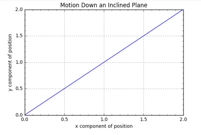
and the energy

was very well conserved.
These good results failed to hold when the shape of the wire was made parabolic. The resulting motion stayed on the parabola for a short time but eventually departed from the constraint by dropping below
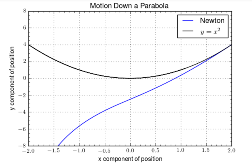
while simultaneously showing a large deviation
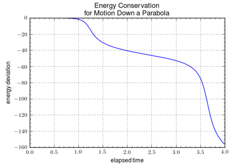
from the initial energy.
The situation was no different for other geometeries tried. The problem seems to lie in the fact that the normal force is unable to respond to numerical errors. As the constraint begins to be violated, the wire is unable to conjure additional force to enforce it. The Newton method, while attractive from its simplicity, is simply inadequate for working with all but the most trivial of constraints.
The usual way of addressing this problem is to eliminate one degree of dynamical freedom. Either $$x$$ or $$y$$ has to go and the conventional approaches seem to favor $$x$$ as the parameter that stays. Again, there are several ways to effect this change but in this case both are worth examining.
In the first method, Newton’s equations are used to eliminate the $$y$$ in favor of $$x$$ by combining their equations of motion by first expressing
\[ -\frac{\ddot x}{g f’} = \tau \]
and then by inserting the left-hand side into the $$y$$ equation yielding
\[ \ddot y + g = -\frac{\ddot x}{f’} \; .\]
Solving this to give
\[ \ddot x = -f'(\ddot y + g) \]
and then using
\[ \dot y = \frac{df}{dx} \dot x = f’ \dot x \]
and
\[ \ddot y = f’ \ddot x + f” \dot x^2 \; . \]
The final equation, after substitution for $$\ddot y$$ has been made and $$\ddot x$$ has been isolated, is
\[ \ddot x = – f’ \tau (g + f” \dot x^2 ) \; .\]
In the second method, the constraint is put into the Lagrangian before forming the Euler-Lagrange equations. The resulting Lagrangian becomes
\[ L = \frac{1}{2} m (1 + f’^2) \dot x^2 – m g f \; . \]
The conjugate momentum is
\[ p_x = m (1 + f’^2) \dot x \; \]
and the resulting Euler-Lagrange equation is
\[ m (1+f’^2) \ddot x + 2 m f’ f” \dot x^2 – m f’ f” \dot x^2 + m g f’ = 0 \; . \]
Simplifying a bit yields
\[ \ddot x = – f’ \tau (g + f” \dot x^2 ) \; , \]
which happily is the same equation as obtained from Newton’s laws.
The last step is to solve this differential equation. Rewriting this equation in state-space form gives a simple system to solve numerically:
\[ \frac{d}{dt} \left[ \begin{array}{c} x \\ \dot x \end{array} \right] = \left[ \begin{array}{c} \dot x \\ -f’ \tau(g + f” \dot x ^2) \end{array} \right] \; .\]
Like the original Newtonian system, this one was easily coded up into Python.
def roller_coaster_Lagrange(state,t,geometry,g):
    #unpack the state
    x  = state[0]
    vx = state[1]

    #evaluate the geometry
    f,df,df2 = geometry(x)
    tau      = 1.0/(1.0+df**2)

    return np.array([vx,-df*tau*(g+df2*vx**2)])
The constraint is always honored since $$y$$ is obtained after the fact from $$x^2$$.
In addition, the conservation of energy

shows that there wasn’t any error in either the theory or the numerical implementation.
However, the key question is, does the solution accurately capture the motion by correctly placing the bead at $$(x,f(x))$$ at the correct time? There is no easy way to answer this question. The plot of the $$x$$ component as a function of time
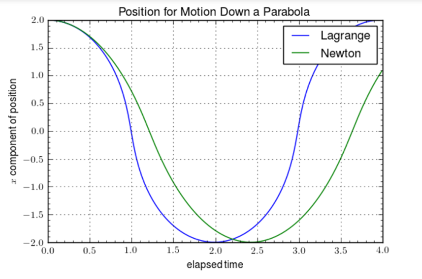
certainly suggests that the Lagrange implementation is correctly capturing not just the dynamics but also the kinematics. That said, a more complete justification will have to wait for another time and another post.