Last month’s blog presented the prototype ‘algorithm’ for relating macroscopic transport properties (e.g., the diffusion coefficient) to their microscopic mechanical attributes (e.g., the mean free path).  This post extends the analysis by giving an elementary expression for relating viscosity and heat conduction to the mean free path, mean speed, and related molecular terms.

Viscosity

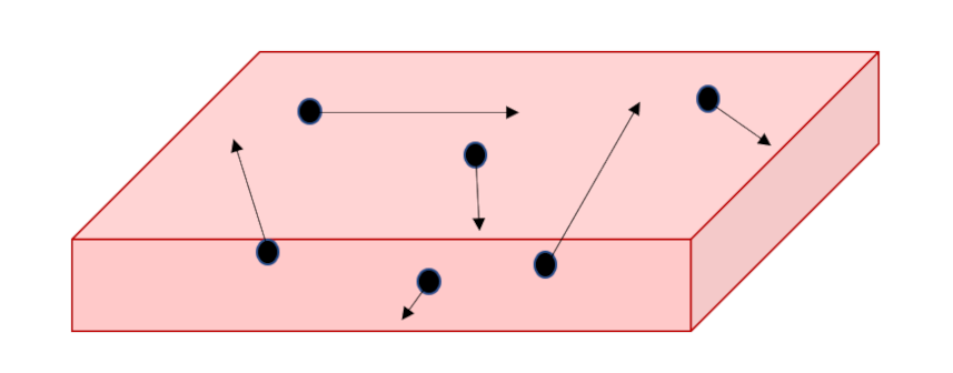
Viscosity as a macroscopic physical phenomenon has been discussed in previous blogs (here and here) and so only short summary will be provided here.  The basic idea is that flow is often fixed or stagnant on a one surface while moving on another.  This is the essential point that Prandtl realized in his concept of boundary layer flow.  The prototypical example is the flow is shown in the figure below where some fluid is forced to flow in the $x$-direction between two plates, separated by a distance $w$ in the $y$-direction, by moving the top plate with a velocity ${\vec u} = U {\hat x}$ with respect to the bottom plate which remains fixed.

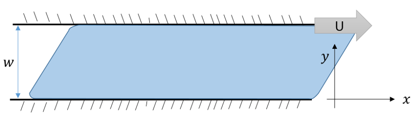
The $x$-component of the fluid’s velocity $u_x$ varies as a function of $y$ and the usual definition of the stress in the problem relates it to the velocity gradient

\[ d_{xy} =  \mu \frac{\partial u_x(y)}{\partial y} \; . \]

The physical meaning of the stress is that $d_{xy}$ is the amount of momentum $p_x$ in the $x$-direction transported across any plane in the $y$-direction, which we will call $p_{xy} = – d_{xy}$ (with an appropriate change in sign to account for difference between a force acting on the fluid and the reaction of the fluid itself).

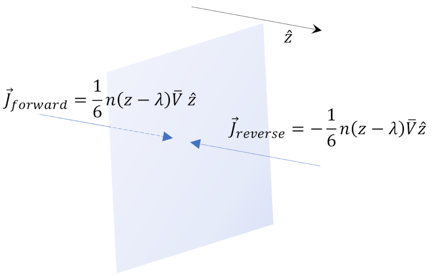
Again, using the Reif’s argument $1/6$ of the molecules will be crossing some plane $y=Y$ in the upward direction and $1/6$ of them will crossing downward.  Assuming the molecular mass as $M$ and the number density as $n$, the difference in momentum is

\[ p_{xy} = \frac{1}{6} M n {\bar V} \left[ u_x(y – \lambda) – u_x(y + \lambda) \right] = – \frac{1}{3} M n \frac{\partial u_x}{\partial y} \lambda \; . \]

Comparing the two expressions gives the viscosity in terms of the microscopic parameters as

\[ \mu = \frac{1}{3} M n {\bar V} \lambda = M n D \; . \]

As with all these types of results, this one should be taken with a grain of salt regarding the numeric factor.  Other authors also get this $1/3$ but they do so using quite different ways of ‘averaging’ across the populations.  Nonetheless, the functional dependence of the viscosity on the microscopic parameters is correct and, in this case, the analysis of this dependence leads to some interesting conclusions.

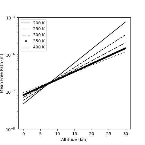
The first thing to note is that Reif expresses the mean free path generally as

\[ \lambda = \frac{1}{\sqrt{2} \sigma n } \; , \]

where $\sigma$ is the generic cross-section, which takes the value $\pi d^2$ for hard sphere collisions giving the expression derived earlier.  This generalization will prove useful in a bit but first let’s look at using this formula for the mean free path explicitly for viscosity.  Putting these together gives an expression for the viscosity

\[ \mu = \frac{1}{3 \sqrt{2} \sigma} M {\bar V} \; \]

that may be quite surprising.  The amount of viscosity delivered by a gas is independent of density, at least over a wide range of values for the physical parameters that enter into this theory.  The limitations occur in the limits of a very small mean free path, in which the gas molecules are nearly always colliding with each other, or when the mean free path is larger than the physical size of the experiment.  Kittel and Kroemer, in their book Thermal Physics, cite a quote from Robert Boyle in 1660 as reading

Before pressing on with more physics, it is worth noting that there are two satisfying things about the above quote.  The first is that Boyle was scrupulous enough to report the null result of performing this experiment; a sentiment that bucks the trend of modern science where only ‘breakthroughs’ are reported.  Second, it is refreshing to hear the ‘snark’ that Boyle conveys on his own behalf. 

Finally, Reif presents how the viscosity changes as a function of temperature.  There is an obvious dependence of speed through the explicit appearance of ${\bar V} \propto T^{1/2}$ in calculating the viscosity.  And, if the collision process were accurately modeled in terms of hard spheres this would be all there was to the dependence.  However, the scattering cross section is, generically, a function of speed since the underlying forces (i.e., Coulomb scattering) have a stronger influence on the particle when it is moving slowly.  This is where the relaxation of the hard sphere scattering assumption becomes relevant as the scattering cross section becomes a function of speed, which, in turn, is a function of temperature in the general case.  Thus, in the general case

\[ \mu = \mu \left[ {\bar V}(T), \sigma ( {\bar V}(T)) \right] \; \]

leading to an overall dependance that Reif cites going as

\[ \mu \propto T^{0.7} \; . \] An interesting implication of this functional dependence (with or without the extra, implicit temperature dependence coming through the effective cross section) is that the viscosity of a gas increases with increasing temperature, which is the exact opposite effect as is active in the vast majorities of liquids.

This month’s and the next two month’s blogs mostly follow Chapter 12 in Fundamentals of Statistical and Thermal Physics by Frederick Reif with some occasional input from (and comment on) other resources.  The primary aim of this post is to show how a very simplistic theory can put the mean free path to use in non-equilibrium situations to make a connection between macroscopically observing bulk transport and the underlying microscopic mechanical motions.

The three cases we will look at are the macroscopic effects of: 1) self-diffusion, which involves the transport of mass, 2) fluid viscosity, which involves the transport of momentum, and 3) heat conduction, which involves the transport of energy.  This order follows the common order used in continuum mechanics for following bulk effect and the corresponding equations in that context are: 1) mass continuity, 2) Cauchy momentum equation, and 3) energy equation.

It is important to stress, that each of these computations is done without regard to the velocity distributions beyond what has already been employed to calculate the mean speed ${\bar V}$ and the mean free path $\lambda$.  Thus, the results that are obtained need to consumed with some care.  The functional dependence of the macroscopic terms on the underlying mechanical analogs is expected to be correct by the overall numerical factor will likely be off by up to a factor of 3 or 4.  This situation is very similar to those discussed in previous blogs concerning which of the statistically significant speeds (most probable, mean, or RMS) should be used in any computation. 

This blog will focus on self-diffusion as the model problem since the other two (viscosity and thermal) follow in much the same way.

Self Diffusion

In Reif’s treatment of self-diffusion, he considers a substance consisting of similar molecules where some subset of them is tagged so that they are observationally distinguishable but (though he doesn’t quite say this) their distinguishability doesn’t affect their mechanical motion.  The mechanism he proffers is that they emit some sort of nuclear radiation that, ostensibly, doesn’t change the mass, but a fluorescence, for example by Raman spectroscopy, might have been a better choice.  Regardless, it seems that he is trying to avoid the situation in which the mass concentration $\rho_m$ varies by constructing a scenario in which only the number concentration $n$ does, ostensibly to avoid bulk motion due to macroscopic flows (i.e., the pressure is uniform). 

Once the molecules have been tagged, he constructs a scenario in which the number density is uniform in the $x$ and $y$ at any fixed value of $z$ but which varies as $z$ does.  As a result, the number density depends on position and time so that $n = n(z,t)$.  There is now a corresponding number density flux ${\vec J} = J_z(z,t) {\hat z}$ in the $z$-direction.  Macroscopically, we assume that since $J_z$ is non-zero when there are differences in the number density, then a linear relationship of the form  

\[ J_z = – D \frac{\partial n}{\partial z} \; , \]

will be adequate provided the gradients are small in some sense.  This relationship is a specific example of Fick’s law

\[ {\vec J} = – D \nabla n \; \]

and $D$ is the self-diffusion constant.  Support for so naming $D$ comes from the fact that if we take the divergence of both side of Fick’s law and the use number continuity equation

\[ \frac{\partial n}{\partial t} + \nabla \cdot {\vec J} = 0 \; \]

to eliminate $\nabla \cdot {\vec J}$ we get

\[ -\frac{\partial n}{\partial t} = -D \nabla^2 n \; , \]

which is the classical diffusion equation.  This classical form, which is well-known, depends on the assumption that $D$ has no spatial dependence; an assumption that is usually stated but not justified.  The elementary transport theory that Reif presents gives a rationale for this assumption and a mechanism to explore for when and how it might break down.

Now consider any plane whose normal is parallel to ${\hat z}$ in between the boundaries with the least and the most concentration of the tagged molecules

Reif argues that $1/6$ of the particles are heading in any of the 6 cardinal direction of $\pm {\hat x}$, $\pm {\hat y}$, and $\pm {\hat z}$.  The forward and reverse number density fluxes, relative to crossing the plane in the +$z$-direction, are given by

\[ {vec J}_{forward} = \frac{1}{6} n(z-\lambda) {\bar V} {\hat z} \; \]

and

\[ {\vec J}_{reverse} = -\frac{1}{6} n(z + \lambda) {\bar V}{\hat z} \; .\]

Note that the mean free path comes in by linking the flux crossing the plane with the number density at a point $z \pm \lambda$ away from which represents that flux originates.  In other words, the molecules that are crossing the plane at $z$ are carrying information from a region one mean free path away, since they will, on average, have suffered no collisions (i.e., interactions) in their travels from that region. 

The $z$-component of the number density flux is then

\[ J_z(z) {\hat z} = {\vec J}_{forward} + {\vec J}_{reverse} \; \]

or

\[ J_z(z) = \frac{1}{6} {\bar V}  \left[ n(z-\lambda) – n(z + \lambda) \right] = -\frac{1}{3} \lambda {\bar V} \frac{\partial n}{\partial z} \; .\]

Comparing the macroscopic expression arising from Fick’s law to this one we arrive at

\[ D = \frac{1}{3} \lambda {\bar V} \; .\] It is interesting to note that in both Kittel’s and Kromer’s book Thermal Physics and in Ashley Carter’s Classical and Statistical Thermodynamics one finds more complicated arguments about averaging over directions and distances to get the leading numerical factor of $1/3$ in the above relation.  I find each of the arguments personally difficult to follow; particularly problematic is that there is a strong linkage between the mean speed, the direction of motion, and the mean free path that leads to a ‘double average’ that ends up resulting in the same wrong numerical factor out front.  As discussed above, the value of $1/3$ can be expected to be good only to a factors on the order of unity.  Reif’s presentation, which simply asserts an intuitive $1/6$ for each of the $6$ cardinal direction, seems far more understandable and concise.

In the last post, we established that the mean free path of a particle, the average distance that the particle travels before suffering a collision with another particle is given by

\[ \lambda = \frac{1}{(N_{rel}/N_{avg}) \pi d^2 n} \; , \]

where $d$ is the characteristic diameter of the particle (i.e., diameter of a bounding sphere) and $n$ is the number density, which depends on temperature and pressure through the ideal gas law .  The factor $N_{rel}/N_{avg}$ is a numerical factor that represents the ratio between the relative speed between the two particles and the average speed of a particle in the gas.  It should be remembered that not all authors agree on which of these statistically significant speeds – mean, most probable, and RMS – should be used in computing the mean free path, so the ratio $N_{rel}/N_{avg}$ can take on values of $\sqrt{2}$, $\sqrt{8/\pi}$, and $\sqrt{3}$, respectively.  While it is important to have rigor and clarity in the analysis and it would be ideal for everyone to agree on the expression, there is little physical impact in choosing one over the other as there is currently no way to independently measure the characteristic diameter of the particle.  Since it is the product of $d^2 (N_{rel}/N_{avg})$ that matters, adjustments to one can be compensated with an appropriate adjustment to the other.  As a result, we’ll take as given the more common value for $ N_{rel}/N_{avg} = \sqrt{2}$.

It is useful to get some sense of the numbers involved for the mean free path in typical terrestrial situations.  To that end, we’ll look at the value of the mean free path for air as a function of altitude from sea level upwards using a crude scale height model of the atmospheric density (see also Kinetic Theory 2 – Maxwell-Boltzmann Distribution).

Atmospheric density in a scale height model is given by

\[ n = n_0 exp \left( – \frac{m g z}{k_B T} \right) \equiv n_0 exp \left( – \frac{z}{H} \right) \; , \]

where $n_0$ is the density at sea level, $z$ is the height in the atmosphere, $H = m g/k_b T$ is the scale height parameter that only depends on the average molecular mass, $m$, of the atmosphere, which is the weighted average mass of molecular nitrogen and oxygen (assumed to be the only components in this abbreviated model) and the temperature $T$; $k_B = 1.38 \times 10^{-23} \, J/K$ being Boltzmann’s constant and $g = 9.8 \, m/s^2$ being the standard gravitational acceleration at sea level.  This exponential form results by assuming that the temperature is constant.  While this assumption is rather poor in fine details, we will use it due to its extreme simplicity.

To get the molecular mass of the air, start first with the molar mass of molecular nitrogen $N_2$ and molecular oxygen $O_2$, whose values are $28 \, amu$ and $32 \, amu$, respectively.  Using the value Avogadro’s number $N_A = 6.022 \times 10^{23}$, the molecular masses (in kilograms) for each of these molecules are: $M_{N_2} = 4.65 \times 10^{-26} \, kg$ and $M_{O_2} = 5.31 \times 10^{-26} \, kg$.  Combining these according to their relative occurrence in atmosphere ($N_2$ at 78% and $O_2$ at 22%) yields the weighted molecular mass of $m = 4.81 \times 10^{-26} \, kg$, which gives a ratio of scale height to temperature of

\[ \frac{H}{T} = 29.5 \, m/K \; .\]

Assuming that the pressure at sea level is one atmosphere ($P_0 = 101325 \, Pa$), the density at sea level is then obtained from the ideal gas law as

\[ n_0 = \frac{P_0}{k_B T} \; , \]

which numerically has the value $n_0 = 2.45 \times 10^{25}/m^3$.

The only remaining piece is the molecular diameter of air which is again a weighted average of the molecular diameter of $N_2$ and $O_2$ which we take to be $364 \, pm$ and $346 \, pm$, respectively,   based on the values listed in Wikipedia for kinetic diameters.  The resulting weighted average gives a molecular diameter of $360 \, pm$ for air.

At a temperature of $T = 27 \, C = 300 \, K$, the mean free path at sea level is $\lambda = 70.9 \, nm$, which, while very small, is still some 200 times larger than the molecular diameter of air.  This means that the assumption underlying kinetic theory – that the particles only interact via direct collision and that those collision take place pairwise – is well supported. 

A related but equally important parameter is the collision time.  The collision time, which is the average time between any two collisions, is related to the mean free path by

\[ \tau = \frac{\lambda}{v_{avg}} \; , \]

where the average speed is given by $v_{avg} = \sqrt{8 k_B T/\pi m}$.  For the $T = 300 \, K$ case above, the corresponding collision time is $\tau = 150 \, ps$.  This value will become more important latter in understanding the collision operator in the Boltzmann equation.

Of course, we can expand these results to various altitudes above the Earth using our scale height model.  The following plot shows the variation in mean free path as a function of altitude for various temperatures.

To get an idea of the accuracy of this model, one can compare its prediction for the mean free path to those from U.S. Standard Atmosphere.  At an altitude of $11 \, km$, the standard atmosphere lists the pressure as $P_{11} = 22632.1 \, Pa$ with a corresponding temperature of $T_{11} = 216.65 \, K$.  Using the ideal gas law, the corresponding number density is $n_{11} = 7.57 \times 10^24 /m^3$ resulting in a mean free path $\lambda_{11} = 2.3 \times 10^-7 \, m \approx 0.2 \mu m$, which is roughly the value predicted by the various models.  At $32 \, km$ a similar computation yields $\lambda_{32} \approx 6 \, \mu m$, which agrees with a scale heigh model to within a factor of 10.  Finally, it is interesting to note that at an altitude of $71 \, km$ (the last fully-listed value) the mean free path is approximately $\lambda_{71} \approx 1 mm$, which makes it on the scale easily seen by the eye (if the eye could actually see the molecule).

Having explored some of the numerical properties of the Maxwell-Boltzmann distribution and the various statistically significant speeds (RMS, most probable, mean), we now turn to the idea of the mean free path and the corresponding collisional frequency.  Since the basic idea of kinetic theory is the mechanical interpretation of macroscopic thermodynamics it is natural to ask about what can be said statistically about the how far, on average constituent particles (e.g., gas molecules) travel before they collide with each other (mean free path) or how often they suffer a collision (collisional frequency).

While the notion of the mean free path is simple enough, its computational form is difficult to come by.  The reason for this is that it depends on one unknown parameter, the characteristic size of a particle.  Typically, whether warranted or not, the particles are, for mathematical simplicity, assumed to be spherical and the so the characteristic size can be thought of as the radius of the bounding sphere into which the particle just fits.

The second complication is that the particles are all moving with various speeds distributed according to the Maxwell-Boltzmann distribution and it isn’t, a priori, obvious whether the mean free path depends on one of the statistically significant speeds or on the distribution as whole.

The content of this post follows, in certain areas, the discussions in Physics by Halliday and Resnick, Classical and Statistical Thermodynamics by Carter, and the Youtube video Mean Free Path by Steven Stuart for Physical Chemistry.  All three agree that the first place to start is by focusing on one particle that is allowed to move within a frozen background of the rest.

Since each particle has a characteristic radius $r$ (and mass $m$), a collision will occur when any two particles are a distance $2r$ from each other. 

Mentally, we can then throw away the bounding sphere around each of the frozen particle, replace the bounding sphere around the mobile particle with one twice as large, and then ask how many particle centers are contained in the cylindrical volume swept out as the mobile particle moves.

The cross-sectional area of this cylinder is $A = \pi (2r)^2$.  If the mobile particle moves a distance $\lambda$, then the volume is

\[ Vol = \lambda A = \lambda \pi 4 r^2 \; . \]

The average number of frozen particle centers that fall within this volume, $N_c$, depends on the number density as

\[ N_c = Vol \cdot n = \lambda \pi 4 r^2 n \; .\]

By definition, the mean free path is the distance, on average, a particle moves before suffering its first collision.  Setting $N_c = 1$ then gives the first estimate as

\[ \lambda = \frac{1}{4 \pi r^2 n}  = \frac{1}{\pi d^2 n} \;  , \]

(where $d = 2r$) which is the result that all three references agree on.

This result can only be justified under the original assumption of one mobile particle moving in a fixed background of all the others being anchored in place.  So, while the above result is dimensionally correct (i.e., the dependence on $(d^2 n)^{-1}$) the prefactor might be different. 

To get a sense of how this prefactor might differ, Halliday and Resnick actually argue for the above result differently.  They assign the mobile particle a speed $v$ and argue that the length it travels in elapsed time $t$ is $vt$.  The total number of collisions is again $\pi d^2 n v t$ and the ratio of these two expressions gives the mean free path

\[ \lambda = \frac{v t}{\pi d^2 n v t} \; . \]

Of course, with the assumption of a single mobile particle, the speeds in the numerator and denominator are identical and can be cancelled out giving the expression derived earlier.  But once we free the previously anchored-in-place particles to move, one must distinguish between the speed in the numerator, which is the “average” speed with respect to the lab (i.e., with respect to the walls of the enclosure) while the speed in the denominator is the speed of the particle we are focusing on relative to the others.  The mean free path now can be written as

\[ \lambda = \frac{v_{avg}}{\pi d^2 n v_{rel}} \; . \]

This argument is a bit subtle and it’s open to interpretation, at this point, which of the statistically significant speeds corresponds to $v_{avg}$ and it is for this reason that not every text agrees on exactly how to determine the ratio of $v_{avg}/v_{rel}$. 

At this point, it is worth reminding ourselves that all the statistically significant speeds, $v_{ss}$, take the form of

\[ v_{ss} = N \sqrt{\frac{k_B T}{m}} \; , \]

where $N = \sqrt{2}$ for most probable, $N = \sqrt{8/\pi}$ for mean, and $N = \sqrt{3}$ for RMS. (It seems the best mnemonic is that $N^2$ is 2, 2.5, and 3, since $8/\pi$ is approximately 2.5 with only a 1.9% error.  The ordering from most probable to mean to RMS is best remembered by just remembering that the Maxwell-Boltzmann distribution has a long tail to the right.)

Thus, we can eliminate a common factor of $\sqrt{k_B T}{m}$ from the numerator and denominator to arrive at

\[ \lambda = \frac{1}{(N_{rel}/N_{avg}) \pi d^2 n} \; .\]

While he doesn’t reduce to the analysis as has been done here, Stuart points out that the resulting expression for the mean free path should have some traces of the speed lingering around when everyone is moving.  He gives two examples in which all the particles have the same speed.  He argues if all the particles are moving coherently in the same direction, then the relative velocity is zero and there will be no collisions.  Alternatively, if one of them is moving oppositely to the others, the number of collisions for this one particle must be double what was predicted by the naïve result.  This is the same argument given in Halliday and Resnick.  Stuart then goes on to derive the correction as follows.

First look at the relative velocity between particles A and B such that

\[ {\vec v}_{rel}  = {\vec v}_A – {\vec v}_B \; .\]

Squaring both sides and averaging over all pairs of particle A and B gives

\[ \langle v_{rel}^2 \rangle = \langle v_{A}^2 \rangle + \langle v_{B}^2 \rangle – 2 \langle {\vec v}_A \cdot {\vec v}_B \rangle \; .\]

Since we envision a large number of particles, the last term averages to zero and we are left with

\[ \langle v_{rel}^2 \rangle = 2 \langle v^2 \rangle \; \]

or

\[ v_{rel,RMS} = \sqrt{2} v_{RMS} \; .\]

With this result, $N_{rel}/N_{avg} = v_{rel,RMS}/v_{RMS} = \sqrt{2}$ and the expression for the mean free path is

\[ \lambda = \frac{1}{\sqrt{2} \pi d^2 n } \; .\]

Interestingly, this is not the expression derived by Carter.  In Sec. 11.7, he states

Frankly, it isn’t quite clear what he means, and the best interpretation seems to be that the relative speed is $\sqrt{2}$ larger than the mean speed (the extra factor most likely due to considerations similar to the above) the while the average speed is identified with the most probable speed (an assumption further supported by his use of the most probable speed in calculating the collision frequency).  With these assumptions the ratio

\[ \frac{v_{avg}}{v_{rel}} = \frac{\sqrt{2 k_B T/m}}{\sqrt{2}\sqrt{8/\pi k_B T/m}} = \frac{1}{\sqrt{8/\pi}} \; .\]

In the end, this minor distinction ($\sqrt{2}$ vs. $\sqrt{2.5}$) doesn’t matter (beyond clarity and pedagogy) since the there is no way to know, with certainty, what the particle diameter $d$ actually is and these formulae are usually used to infer $d$ by measuring $\lambda$. 

Next column will look at some characteristic values and the corresponding question of the collision frequency, where, again, we’ll have to wrestle a bit with which of the statistically significant speeds to use.

In this post, we explore some of the physical implications of the Maxwell-Boltzmann speed distribution

\[ f(v) = 4 \pi \left( \frac{m}{2 \pi k_B T} \right)^{3/2} v^2 \exp \left( – \frac{m v^2}{2 k_B T} \right) \; \]

derived in the previous post.

The first thing to note is that the decaying exponential favors lower speed (in the limit as $v \rightarrow \infty$, $f(v) = 0$) while the factor of $v^4$ favors higher ones ($f(v=0) = 0 $).  As a result, we expect that there is a peak in the distribution somewhere between these two extremes.  To verify this, we can plot $f(v)$ for the case where $m$ is the mass of a nitrogen gas molecule ($m_{N_2} \approx 28 Da$, where $1 Da \approx 1.66 \times 10^{-27} \, kg$) and the temperature is $300 K$, corresponding, roughly, to room temperature.

There is a distinct peak, which can be estimated by eye, at approximately $420 \, km/s$.  This value is of the order-of-magnitude of the RMS speed given by

\[ v_{RMS} = \sqrt{ \frac{3 k_B T }{m_{N_2}}}  = 510.77 \, km/s \; ,\]

but is substantially smaller by about $20 \, \%$.  The exact value at the peak, which corresponds to the most probable value, comes from finding the maximum of the distribution in the usual way.  First we differentiate the distribution with respect to $v$ to get

\[ \frac{d f(v)}{d v} = 4 \pi \left( \frac{m}{2 \pi k_B T} \right)^{3/2} \left( 2 v – \frac{ m v^3}{k_B T} \right) \exp \left( – \frac{v^2}{2 k_B T} \right) \; . \]

Setting this expression to zero and solving for $v$ yields the most probable speed

\[ v_{mp} = \sqrt{\frac{2 k_B T}{m} } \; .\]

Plugging in the numerical values used above gives $v_{mp} = 417.04 \, km/s$, which is consistent with eyeball estimate of $420 \, km/s$.

The final speed of interest is the average speed defined by

\[ v_{ave} = \int_0^{\infty}\, dv \,  v f(v) \; .\]

Ordinarily, the odd moment of any Gaussian-like distribution would be zero (e.g., the average of any component of the velocity would be zero – see last post) but since the speed is confined to the interval $[0,\infty)$, the integral yields a finite value.  To get that moment, we start with

\[ J_1 = \int_0^{\infty} \, v e^{-qv^2} dv = \frac{1}{2} \int_0^{\infty} \, d(v^2) e^{-q v^2} \; .\]

Substituting  $w = v^2$ yields a simple integral

\[ J_1 = \frac{1}{2} \int_0^{\infty} \, dw e^{-q w} = \frac{1}{2q} \; . \]

Higher order moments come by differentiation with

\[ J_3 = \int_0^{\infty} v^3 e^{-q v^2} dv = -\frac{d}{dq} \int_0^{\infty} v e^{-q v^2} = -\frac{d}{dq} \frac{1}{2q} = \frac{1}{2q^2} \; ,  \]

which, up to some constants, is the desired result.

Using this result, we arrive at the expression

\[ v_{ave} = 4 \pi \left(\frac{m}{2 \pi k_B T}\right)^{3/2} \frac{k_B T}{m} = \sqrt{ \frac{8 k_B T}{\pi m}} \; .\]

Plugging in the numerical values used above gives $v_{ave} = 470.58 \, km/s$, which falls between the most probable and the RMS speeds.  We can annotate the graph with these three lines to draw out the distinctions

and we can note that the average speed is about $12.8 \, \%$ higher than the most probable speed while the RMS speed is $22.5 \, \%$ higher.

The final point to be explored is how the curve shifts as a function of temperature.  Since all the speeds have the same functional form, differing only in the numerical coefficient, it is straightforward to see that each speed scales as $\sqrt{T}$.  However, the overall shape of the curve can be a little surprising, which the following plot illustrates by looking at broad range of temperatures.

As the temperature increases, the distribution tends to being more symmetric by shifting right, effectively eating into the long tail. 

Of course, the Maxwell-Boltzmann distribution is physically unrealizable as there is always a finite probability for having a speed equal or greater to the speed of light.  But this is of little concern as very little of the distribution is found at these higher speeds.  For example, the vast majority of the distribution is found below $2000 \, km/s$, which is $ < 0.01 c$, even at $T = 1000 K$. 

One of the great accomplishments of 19th-century physics was the creation of the Maxwell-Boltzmann distribution of molecular speeds in a gas. There are many ways to derive this fundamental relationship but there are two that stand out due to their mathematical brevity and physical content.

The first one is Boltzmann’s very clever argument based on relating hydrostatic equilibrium to the ideal gas equation of state. This argument introduced itself to me in the pages of Physics, 3rd Edition by Halliday and Resnick but the presentation given here has been modified to bring the physical logic to the forefront.

The argument goes as follows: We want to know the velocity distribution of the molecules making up a gas, say air to be concrete, and we don’t have a way to measure this distribution (below we’ll talk about methods that have been subsequently invented). We imagine that we can extract a slab of air, of thickness $dz$ at a specified instant at a uniform temperature $T$. The molecules will be moving in random directions and with random speeds.

Since gravity is acting along the $z$ direction, we can use it as an analyzer since we can link the height obtained by an individual molecule to its kinetic energy, which then links to the initial speed. Since we won’t care, at this stage, about the horizontal components of each random motion, we’ll imagine that we’ve set them to zero and we’ll concentrate only on the vertical motion.

Since we seek the stationary distribution, we can further envision that there is a floor off of which the molecules can bounce keeping the supply of particles constant. These extracted particles will then separate into a thicker slab with the more energetic of them being able to obtain greater values in $z$ while the slower ones will remain at smaller heights; a vertical gradient in density will result solely due to differences in speed.

The next point in Boltzmann’s argument is point out that we know how to macroscopically describe such a density gradient in an isothermal atmosphere using fluid mechanics and thermodynamics. The first step is to start with the Euler equation (link) under the external influence of gravity

\[ \rho \frac{d}{dt} {\vec v} = \, – \nabla P + {\vec F}_g \; ,\]

where $\rho$ is the mass density. Specializing to stationary equilibrium in one dimension (called $z$, in keeping with the above argument):

\[ 0 = \, – \frac{d}{dz} P – \rho g \; . \]

The next step with a modification eliminating the mass density $\rho$ in favor of the number density $n$, to which it is proportional with the constant of proportionality being the molecular mass $m$: $\rho = m n$. The next step assumes the ideal gas law $P = n k_b T$ to eliminate the pressure giving

\[ \frac{dn}{n} = \, – \frac{m g}{k_B T} dz \; . \]

Since we’ve stipulated an isothermal profile (this assumption does not hold for the atmosphere as a whole it does for any local portion and that is all that is needed for Boltzmann’s argument to work), this differential equation readily solves to

\[ n(z) = n_0 \exp \left( – \frac{m g z}{k_B T} \right) \; , \]

where $n_0$ is some constant.

The next point in his argument is to relate the gravitational potential energy to molecules kinetic energy, thereby eliminating $z$. This is the point where the notion that the particles bounce vertical to different heights based on their initial velocities comes into play. This video by tec-science has a nice illustration of the physics. The final form for the number density as a function of $v_z$ is

\[ n(v_z) = n_0 \exp \left( – \frac{m v_z^2}{2 k_B T} \right) \; . \]

Demanding this function be normalized gives the distribution function

\[ f(v_z) = \sqrt{\frac{m}{2\pi k_B T}} \exp \left( – \frac{m v_z^2}{2 k_B T} \right) \; . \]

Boltzmann’s final point is that, although gravity was an essential part for getting started, now that it has been eliminated the form of $f(v_z)$ also applies to the $x$- and $y$-directions. The full three-dimensional form is

\[ f({\vec v}) = \left( \frac{m}{2\pi k_B T}\right) \exp \left( – \frac{m {\vec v}\cdot {\vec v}}{2 k_B T} \right) \; .\]

A different, physical approach is given by Carter in his Classical and Statistical Thermodynamics. To the usual kinetic theory assumptions, he adds the very plausible idea that in a dilute gas, only binary collisions are important. Similar to above, he limits the analysis to a single species of known mass $m$. The conservation of momentum requires

\[ {\vec v}_1 + {\vec v}_2 = {\vec v’}_1 + {\vec v’}_2 \; , \]

where ${\vec v}_1$ and ${\vec v}_2$ are the initial velocities of the two molecules and the primed versions are the final velocities.

Carter points out that kinetic theory predicts that an inverse collision also has to be present taking ${\vec v’}_1$ and ${\vec v’}_2$ back to their unprimed versions in order to have equilibrium. He then assumes that $f({\vec v})$ is the distribution and that the number of collisions between molecules with velocity ${\vec v}_1$ and ${\vec v}_2$ is $\alpha f({\vec v}_1) f({\vec v}_2)$ for some constant $\alpha$. Likewise, the number of inverse collisions must be $\alpha’ f({\vec v’}_1) f({\vec v’}_2)$. As already remarked, in equilibrium

\[ \alpha f({\vec v}_1) f({\vec v}_2) = \alpha’ f({\vec v’}_1) f({\vec v’}_2) \; . \]

The final step involves recognizing that the two collisions, unprimed-to-primed and primed-to-unprimed, are equivalent in the center-of-mass frame (simply switch the arrow heads from in to out) so that $\alpha = \alpha’$.

Since the kinetic energy is conserved, the following constraint applies

\[ v_1^2 + v_2^2 = {v’}_1^2 + {v’}_2^2 \; .\]

After some reflection, one can see that the functional form

\[ f({\vec v}) = A \exp(-q {\vec v} \cdot {\vec v} ) \; \]

fits the bill. This is functionally the same distribution derived from the hydrostatic analysis above, although the values of $A$ and $q$ have not been determined yet. The form of $q$ follows from imposing a consistency constraint with the ideal gas law. Since the ideal gas law doesn’t involve directionality, we’ll find it convenient to construct a related distribution $f(v)$, which gives the fraction of the gas moving with speed $v$. This distribution is related to the velocity distribution by integrating over the angular degrees of freedom in spherical polar coordinates.

\[ f(v) = \int_0^{2 \pi} d\phi \int_{-1}^{1} d(cos(\theta)) v^2 dv A e^{-q {\vec v} \cdot {\vec v}} \\ = 4 \pi v^2 A e^{-q {\vec v} \cdot {\vec v}} \; . \]

Normalizing $f(v)$, over the range $[0,\infty)$, yields the relationship

\[1 = 4 \pi A \left( -\frac{d}{dq} \right) \frac{1}{2} \sqrt{ \frac{\pi}{q} } = A \left( \frac{\pi}{q} \right)^{3/2} \; .\]

Now we demand that the average of the kinetic energy $1/2 m v^2$

\[ \left< \frac{1}{2} m v^2 \right> = \int_0^{\infty} \frac{1}{2} m v^2 \times 4 \pi A v^2 e^{-q {\vec v} \cdot {\vec v}} \; . \]

be equal to $3/2 k_B T$, in keeping with the ideal gas law. Performing the appropriate integral yields

\[ \frac{3}{2} k_B T = \left( -\frac{d}{dq} \right) 2 \pi m A \left( \frac{\pi}{q} \right)^{3/2} = \frac{3 m}{4} A \frac{{\pi}^{3/2}}{q^{5/2}} \; , \]

or

\[ k_B T = \frac{m A}{2} \left( \frac{\pi}{q} \right)^{3/2} \frac{1}{q} \; . \]

Combining this relation with the normalization relation gives

\[ q = \frac{m}{2 k_B T} \; . \]

Another approach involves calculating the pressure and comparing against the ideal gas law also gives

\[ q = \frac{m}{2 k_B T} \; , \]

from which follows the same form as above. A nice derivation of this result comes from Heat and Thermodynamics by Anandamoy Manna.

This final form is

\[ f(v) = 4 \pi \left( \frac{m}{2 \pi k_B T} \right)^{3/2} v^2 \exp \left( – \frac{m v^2}{2 k_B T} \right) \; .\]

This is the famous Maxwell-Boltzmann distribution. In the next post, we’ll explore some of the consequences of this distribution.

Last month’s post marked a logical end to the study of classical thermodynamics.  This month’s post begins the transition from thermodynamics to statistical mechanics by giving a simple treatment of the kinetic theory of gases.  While the mathematical and theoretical sophistication of kinetic theory is quite high, this introductory post will confine itself to an elementary treatment following Physics by Halliday and Resnick but with additional departure points identified.  The results that follow should serve as a baseline for a more realistic presentation to follow.

The aim of kinetic theory is to establish the properties of a gas, most notably the ideal gas law, in strictly mechanical terms.  The three thermodynamic variables of volume, $V$, pressure, $P$, and temperature, $T$, have their ultimate definition in terms of the microscopic movement of the gas molecules.  The volume occupied by the gas should be obviously connected to the density of the gas, but it may be somewhat harder to understand that pressure is a manifestation of the momentum imparted to nearby objects through the collision of the gas with them.  The connection between the temperature and the average kinetic energy per molecule should be even more removed.

Since the ideal gas law finds applications in a variety of physical scenarios from the modeling of galaxies and stars to more terrestrial applications in internal combustion and steam engines and weather and atmospheric modeling, the success of the mechanistic approach of kinetic theory was one of the great triumphs of 19th century physics.  In unearthing these connections we will assume that the ideal gas law is given as

\[ P V = n R T = N k_B T \; , \]

where $n$ is the number of moles and $R$ is the ideal gas constant, which can also be expressed in terms of the Boltzmann constant $k_B$ and Avogadro’s number $N_A$ as $R = k_B N_A$.

The typical textbook story starts with looking a single particle moving within a cubical enclosure of side length $L$.  The confinement to a single particle is not as radical as it may seem at first since this arrangement is logically equivalent to having $N$ particles in the box that don’t interact with each other (i.e., no collisions).  This latter assumption is easy to relax after the derivation and it will be addressed again below.

We envision this single particle to have a mass $m$ and initial velocity ${\vec v}_I = (v_x,v_y,v_z)$.  Let us suppose that the particle is approaching the right-most face perpendicular to the $x$-axis. 

If the particle elastically collides with the wall, its $x$-component of velocity is negated leaving a final velocity ${\vec v}_F = (-v_x,v_y,v_z)$.  The change in particle momentum during the collision is

\[ {\vec p}_{F} – {\vec p}_{I} = m {\vec v}_F – m {\vec v}_I = (-2 m v_x ,0,0) \; .\]

In response, the momentum transferred to the wall is

\[ \Delta {\vec p} = (2 m v_x,0,0) \; . \]

We now follow as the particle strikes the opposite wall, rebounds, and then again strikes the first wall.  The time it takes for this round trip across the enclosure is

\[ \Delta t = \frac{2 L}{v_x} \; , \]

independent of whether or not is strikes the other faces with unit normals not along the $x$-axis.  The force this particle exerts on the right-most wall of the container is the change in momentum imparted at each collision divided the time between collisions and is given by

\[ {\vec F} = \frac{\Delta {\vec p}}{\Delta t} = \frac{(2m v_x,0,0)}{2 L / v_x} = \left( \frac{m v_x^2}{L} \right) \; . \]

With the result for a single particle in hand, we can now imagine the box now filled with $N$ particles each with their own particular value for the $x$-component of the velocity, which we will track with an index: $v_{xi}$.  The pressure due to all of these particles is then the ratio of the total force to the area of the face and is given by

\[ P = \frac{F_x}{L^2} = \frac{m v_{x1}^2/L + m v_{x2}^2/L + \cdots m v_{xN}^2/L  }{L^2} \\ = \frac{m}{L^3} \left( v_{x1}^2 + v_{x2}^2 + \cdots v_{xN}^2 \right) \; .\]

Multiplying the numerator and denominator of the last expression by $N$ gives the pressure in terms of the average $x$-component of the velocity as

\[ P = \frac{m N}{L^3} ( v_x^2 )_{ave} \; . \]

We can express the average $x$-component of the velocity in terms of the average of the speed by first noting that by definition $v^2 = v_x^2 + v_y^2 + v_z^2$ and that since there is nothing special about the $x$ direction (i.e., there is rotational symmetry), the $y$ and $z$ directions must also have the same value.  Combining these two ideas we get that

\[ (v^2_x)_{ave} = \frac{(v^2)_{ave}}{3} \; .\]

Since $L^3 = V$, we can rewrite the pressure as

\[ P = \frac{m N}{3 V} (v^2)_{ave} \; .\]

This last this expression for pressure can be directly compared with the thermodynamic equation of state giving

\[ \frac{N k_B T}{V} = P = \frac{N m v^2_{rms}}{3 V} \; . \]

Eliminating common factors and renaming the average speed, as is traditional, as the root-mean-square speed we get

\[ T = \frac{m N v_{rms}^2 }{3 k_b} = \frac{2}{3} \frac{KE_{rms}}{k_b} \; .\]

The physical meaning we attach to this expression is that the temperature perceived by a thermometer is two thirds of the kinetic energy of the gas moving at $v_{rms}$ scaled by the Boltzmann constant. 

Since we can directly measure temperature much more easily than we can measure molecular speeds, the more common way of presenting this relationship is to express $v_{rms}$ in terms of temperature as

\[ v_{rms} = \sqrt{ \frac{3 R T}{M} } \; ,\]

where the macroscopic parameters of the ideal gas constant $R = k_B N_A$ and molar mass $M$. 

This connection between temperature and kinetic energy is profound but is subject to several questions.

First, what modifications result if inter-particle collisions are accounted for?  It turns out that no modifications are actually needed since the action of a collision will be to switch velocity components between the particles involved in the collision due to the conservation of momentum.  Since we imagine that a whole distribution of speeds is present for each component the statistical average figuring into the pressure remains unchanged.  This argument can also be found in Halliday and Resnick’s first chapter on Kinetic Theory.

Second, and more importantly, what modifications result if the collisions (inter-particle or particle-with-wall or both) are inelastic?  The obvious interpretation is that energy is lost or gained as heat but the clear signposts pointing to this conclusion are not even touched upon in an elementary presentation and aren’t obvious in the simplistic treatment above.  This is the operative question because it carries in its train a host of related questions such as: what if the collision create new particles?  what if the collision is mediated by a field?  what if the collisions are overlaid with a long-range force? and so on.  No doubt, this is where the conservation of momentum plays a starring role but exactly how remains to be seen as we work our way through kinetic theory.

Next month, we’ll look at how the individual particle speed are distributed around $v_{rms}$ by deriving the famous Maxwell-Boltzmann distribution.

This post brings to a close, for the time being, the analysis of classical thermodynamics.  It seems fitting to end with an example that sharpens much of what has been discussed over the past year or so.  Such an example is given by Willis and Kirwan in their article The “Sadly Cannot” thermodynamic cycle.  This two-stroke cycle is a thought-provoking model of a possible heat engine where a naive application of thermodynamics leads one astray.  Finding one’s path back challenges one to think more carefully about what the terms of thermodynamics actually mean. 

Their two-stroke engine consists of two simple thermodynamic processes connected together to form a cycle.  A monatomic gas serves as a working fluid ($\gamma = C_P/C_V = 5/3$). Along the first leg of the cycle the gas decompresses from a volume $V_A$ to a volume $V_B$.  The equation relating pressure and volume during this leg is the linear equation

\[ P = a V + b \; . \]

Along the second leg of the cycle, the gas is adiabatically compressed with the equation relating pressure and volume being

\[ P V^{\gamma} = constant \; . \]

The operating points $A$ and $B$, where the two legs connect, have pressures, volumes, and temperatures of $(P_A, V_A, T_A)$ and $(P_B, V_B, T_B)$, respectively.  Two additional points are called out on the first leg.  The first one, labeled $T_M$ is the point in the decompression leg where the temperature reaches a maximum.  The second one, labeled $Q_R$ is the point where heat flow reverses from flowing into the system to flowing out.  The name of the cycle, Sadly Cannot, is an homage to Sadi Carnot.

To see the magic of the Sadly Cannot cycle, Willis and Kirwan give a typical example.  Given that $P_A = 32 Pa$, $V_A = 8 m^3$, $P_B = 1 Pa$, and $V_B = 64 m^3$, compare the thermal efficiency of this two-legged cycle to that of a Carnot cycle operating between the same two temperature extremes.  Thermal efficiency, \ is defined as

\[ \epsilon = \frac{\textrm{work extracted}}{\textrm{heat supplied}} \; .\]

Let’s start by determining how much work is extracted.  This value will be the sum of the signed areas lying below each curve.  For the linear equation on the first leg, a simple calculation gives $a = (P_A – P_B)/(V_A – V_B) = -31/56 \, Pa/m^3$ and $b = (P_A – a V_A) = 255/7 \, Pa$.  The work done by the gas along this leg is

\[ W_{A \rightarrow B} = \int_A^B P dV = \int_{V_A}^{V_B} (a V + b) dv = \left. \left(\frac{1}{2} a V^2 + b V\right) \right|^{V_A}_{V_B} = + 924 J\; .\]

The positive value of work is consistent with the expansion of the gas against the environment (e.g., a piston) and comes at the expense of some combination of reduced internal energy and heat exchange with the environment. 

Since the second leg is, by construction, an adiabat, the work can be determined immediately from the first law since $\Delta U = Q_{B\rightarrow A} – W_{B\rightarrow A} = -W_{B\rightarrow A}$.  Rather than performing an integral (which is easy enough but not illustrative), we can use the change in internal energy, which is directly related to the change in temperature by $\Delta U = 3/2nR(T_A – T_B)$, to calculate the work.  We can eliminate temperature in favor of pressure and volume by using the equation of state to get $\delta U = 3/2(P_AV_A – P_BV_B) = -288 J$.

Thus the net work done during the cycle is $W_{net} = W_{A \rightarrow B} + W_{B \rightarrow A} = 636 J$.

We now need to calculate the heat transferred between our engine and its surroundings.  We already used the fact that, by construction, $Q_{B\rightarrow A} = 0$ since the second leg is an adiabat.  All we need is $Q_{A\rightarrow B}$.  Here we may be tempted to again use the first law to arrive at the thermal efficiency of the engine arguing this way:  Upon completing an entire circuit of the Sadly Cannot cycle, the gas is now back to the same thermodynamic state from which it started, thus the corresponding change in internal energy is $\Delta U_{net} = $.  Applying the first law then gives

\[ \Delta U_{net} = 0 = Q_{net} – W_{net} \; , \]

or $Q_{net} = W_{net} = 636 J$.  There is nothing intrinsically wrong with the calculation except that it doesn’t help us figure out what the thermal efficiency is and, if we use this value, we come up with the nonsensical value of $\epsilon =1$ in clear violation of one of the many equivalent ways of expressing the second law.

The next step involves answering two questions.  The first is, what went wrong?  The second is, what value should be used for the heat provided?  In short, the answer to what went wrong is simply summarized by the following inequality:

\[ Q_{net} \neq Q_{supplied} \; .\]

The reason these two are not equal is that somewhere along leg 1 heat stops flowing into the system (i.e., being supplied) and starts flowing out (i.e., being shed).  These two values of heat add to form $Q_{net}$, but only the value of $Q_{supplied}$ is used in computing the efficiency of our engine.  The heat shed $Q_{shed}$ is energy given back to us by the process but it is energy with which we can do nothing useful until we feed it back into an engine (either this one or some other).  To calculate $Q_{supplied}$ we need to integrate along leg 1 only to the point $Q_R$ where the heat reverses. 

The heat along leg 1 is obtained from the first law again via

\[ Q = \int \Delta U + \int P dV + constant \; .\]

Since the internal energy only depends on temperature, we can, as above, use the equation of state to get

\[ U = \frac{3}{2} n R T = \frac{3}{2} P V = \frac{3}{2} \left( a V^2 + b V \right) \; . \]

Likewise, the work as a function of state is given by

\[ W = \int \left(a V + b\right) dV = \frac{a V^2}{2} + b V \; . \]

The heat as a function of state is then

\[ Q = 2 a V^2 + \frac{5}{2} b V + constant \; . \]

Setting $dQ/dV = 0$ and solving for V yields

\[ V_R = -\frac{5}{8} \frac{b}{a} = 1275/31 m^3 \; . \]

Plugging this value back into the linear equation relating pressure and volume gives a value of

\[ P_R = -3/8 b = 765/56 Pa \; . \]

The heat supplied is then

\[ Q_{supplied} = Q_R(P_R,V_R) – Q_A(P_A,V_A) \approx 1251 J \; , \]

yielding an efficiency of $\epsilon \approx 0.52$. 

Calculating the efficiency of the corresponding Carnot cycle is also not a simple plug-and-chug.  The maximum temperature occurs somewhere on leg 1 before the heat reversal.  To find it, we recognize the $dU/dV=0$ applied to the expression for internal energy in terms of pressure and volume used above.  Taking the derivative and solving for volume gives a value of $V_H = \frac{-b}{2a}$ at the corresponding pressure of $P_H = \frac{b}{2}$.  The efficiency of the Carnot engine is

\[ \epsilon_{Carnot} = 1 – \frac{T_B}{T_H} = 1 – \frac{nRT_B}{nRT_H} = 1 – \frac{P_B V_B}{P_H V_H} \approx 0.89 \; .\]

In a companion piece entitled The “Sadly Cannot” Thermodynamic Cycle Revisited, Mills and Huston point out that these special points can be obtained by recognizing that the requirements that $dQ/dV=0$ for where the heat reverses and $dU/dV=0$ for maximum temperature mean that the point $Q_R$ falls on an adiabat (since no heat is flowing at that point) and the point $T_M$ on an isotherm (since the temperature is not changing at the point). Along the adiabat $P V^{\gamma} = constant$ and the implicit derivative from this equation can be connected to the explicit linear equation to arrive at the same values for $V_R$ and $P_R$.  Likewise, the same process is used along the isotherm with the only change being to use $PV = constant$. 

It is rare to find such a satisfying example anywhere in physics as the Sadly Cannot cycle is.  Well done, Willis and Kirwan.

The concept of a state in physics is a surprisingly subtle and tricky concept, involving many potential layers of abstraction and encapsulation.  And no other discipline within physics demonstrates this subtly quite as poignantly as does classical thermodynamics. 

Take, for example, a collection of water molecules.  If the collection is empty, that is to say there are no molecules in it, then quantum field theory tells us that the state of the system is described by the vacuum field $| 0 \rangle$ with all of the quantum field operators and ephemeral fluctuations winking into and out of existence present in that description. If the collection holds a single water molecule and we are interested in the vibrational and rotational modes, the ionization and bonding angle, and similar physical quantities then the state is better described by quantum many-body wave function $\Psi (\left\{ {\vec r}_i \right\}, t)$.  If the collection has a small number $N$ of water molecules and we are interested in their interaction with their container and with each other via collisions, then the state comprises the individual positions and velocities ${\bar S} = \left[ {\vec r}_1, \ldots, {\vec r}_N, {\vec v}_1, \ldots, {\vec v}_N \right]$ evolved according to the usual Newtonian laws.  If there are a vast number of water molecules and they are in equilibrium then the state is describe by the partial differential equations governing the thermodynamic functions of density $\rho$, pressure $P$ and temperature $T$ (with the usual extension to hydrodynamics should there be hydrodynamic flows and gradients).

Given the elastic nature of the concept of state, stretching and bending as needed, it should hardly be a surprise that confusion and misuse might arise across the physics community. 

Peter Enders (in an article entitled Gibbs’ Paradox in the Light of Newton’s Notion of State in a letter to Entropy in 2009) argues that the resolution of the Gibb’s paradox – which has been a theme in this column’s analysis of how entropy is defined and understood – lies in the careful consideration of state.

According to Enders’s analysis, the Gibbs paradox arises when one uses what he calls the Lagrange-Laplace concept of state, defined as a collection of “the dynamical variables positions and velocities or momenta of all bodies involved”.  He argues that this notion of state counts the interchange of two “identical” particles as “representing two different states”.

Enders asserts that a Newtonian concept of state produces no paradoxical increase in entropy because

He links the Newtonian state with the Hamiltonian and, thereby, with statistical mechanics and thermodynamics.  In terms of the usual explanation for the factor of $1/N!$ being needed from quantum considerations of indistinguishable particles, Enders says firmly

He summarizes his analysis by saying

Now, it isn’t important to finding Enders’s analysis compelling (although I’ll confess that I do) to appreciate that the logical and conceptual subtleties associated with what exactly is meant by the word state.

This quote, taken from Section 1.5 of Challenges to the Second Law of Thermodynamics by Vladislav Capek and Daniel P. Sheehan, is the theme for this month’s blog providing both an admonition and the capstone of much of the past year’s worth of posts.

Over a year ago (15 months to be more exact – in the post entitled An Invitation to Entropy) I asserted that no physical concept was as poorly understood as entropy.  I based that claim on a similar statement by Swendsen, who presented 9 pairs of contradictory statements about entropy in an article for the American Journal of Physics.  Over the intervening months, this column has explored various ways of looking at entropy and the second law as a way of testing this assertion.  It did this mostly by following the logic of Enrico Fermi’s book Thermodynamics or, a text clearly influenced by it, Ashley Carter’s Classical and Statistical Thermodynamics.

Fermi’s approach (here I also include Carter) had a clear plan of showing the logical equivalence of three different articulations of the second law: Kelvin-Planck, Clausius, and Carnot and then using them (predominantly Carnot’s theorem) to introduce entropy as a state variable, a discovery that was one of the great triumphs of nineteenth century physics. 

This approach is powerful in its cohesion but it is not powerful enough to have persuaded every physicist, or even a majority of them, as to its completeness and universality.  Anyone who doubts that conclusion need only consult Chapter 1 of Capek and Sheehan in which they say “[o]nce established, it settled in and multiplied wantonly; the second law has more common formulations than any other physical law.”  In that chapter, they present an excellent history of the thinking about the second law in order to set the stage for the various challenges that follow.  They also present ‘21’ different expressions of second law along with the assurance that not all of them are logically equivalent.   The following table lists the various ones provided by Capek and Sheehan roughly grouped by the categorization scheme they use.

Capek and Sheehan go to great pains to stress that this list is by no means exhaustive.  They offer the following in way of explaining just why there are so many inequivalent ways of looking at the second law:

In the same chapter they also present 21 non-equivalent definitions of entropy ranging from Clausius’ original statement of $S$ as a state variable to Boltzmann’s notion of relating it to the natural logarithm of the number of microstates to modern quantum and information theoretic points-of-view.  They notes that:

Capek and Sheehan provide a number of insights and thought-provoking (and often witty) points.  They present an excellent critique demonstrating how the ambiguity in the definition of equilibrium state is strongly linked to the level of abstraction one employs in describing nature.  But the primary scientific utility they provide is drawing a clear distinction between the second law and entropy (hence the introductory quote).  Sheehan goes so far as to opine that the concept of entropy, despite its historic and current usefulness, must eventually be abandoned in favor of concepts more in line with the systems being studies. 

Capek and Sheehan have done a great service in compiling this summary and by drawing sharper distinctions in a subject that encourages fuzzy thinking.  I’ll leave this month’s post by quoting them again as the impress on the reader just how far we have to go with understanding nature, thermodynamics, and the second law: