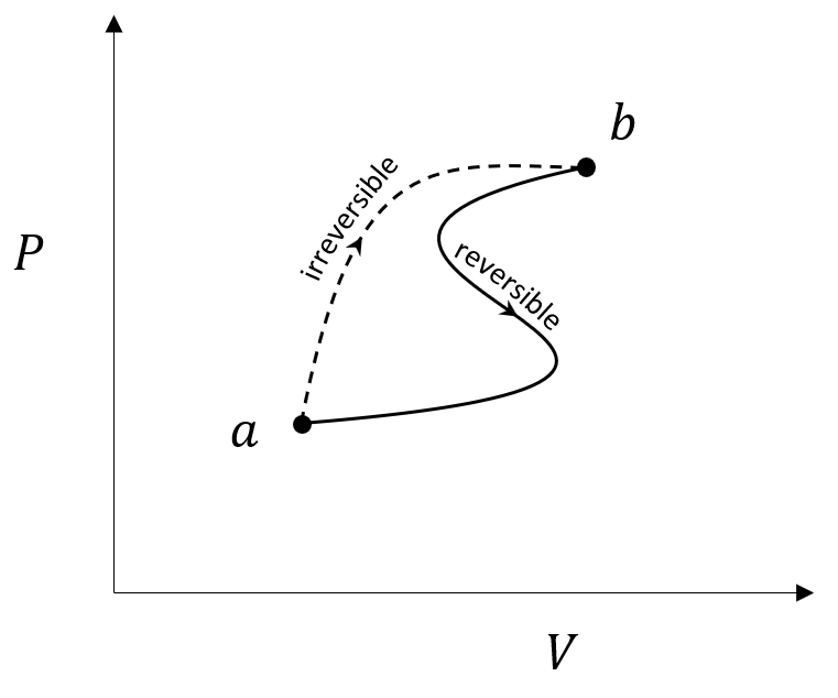
The example of supercooled water from last month’s was instructive both from the perspective of the usefulness of state variables but also from the point-of-view understanding irreversible processes.  However, the effectiveness of the approach was blunted by the fact that the supercooled drop in spontaneously freezing actually had a drop in entropy and not an increase as we would expect from the Clausius inequality.  In order to argue that the ‘sudden freeze’ mentioned in the problem statement was truly irreversible, we had to calculate the change in the entropy of the surroundings and confirm that the total entropy change of the universe (drop and surroundings) was greater than zero: $\Delta S_{uni} > 0$.

The need to look at both the system in question and the surroundings is awkward and inconvenient, especially for the chemist.  Perhaps, no text expresses the distaste for using entropy change directly as sharply and succinctly as Physical Chemistry by J. Edmund White, in which the author has a bolded heading in Chapter 6 which reads “Entropy is not a satisfactory criterion of spontaneity”. 

White argues in that section, that “the practicing chemist needs way to predict…whether a reaction is spontaneous”.  He first notes that originally, scientists thought that if changes in internal energy or enthalpy were negative ($\Delta U_{S,V} \leq 0$ or $\Delta H_{S,P}$ in his notation) these would be good indicators of spontaneous reactions.  He then offers the counterexample of ice at $21 {}^{\circ}C$ spontaneously melting even though the change in either internal energy of enthalpy is clearly positive. 

He then goes on to also reject entropy for the reasons discussed above. In disposing of entropy he remarks that “[a] more useful criterion would depend only on the process or system and would apply under the usual conditions for chemical reactions: constant $T$ and $P$ or constant $T$ and $V$.”

At this point White introduces the two thermodynamic potentials: the Gibbs free energy $G = U – TS – PV$ and the Helmholtz free energy $F = E – TS$ and off he goes.  To understand why, remember that spontaneous processes occur when

\[ \Delta S_{uni} = \Delta S_{sys} + \Delta S_{sur} \geq 0 \; .\]

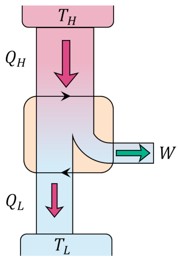
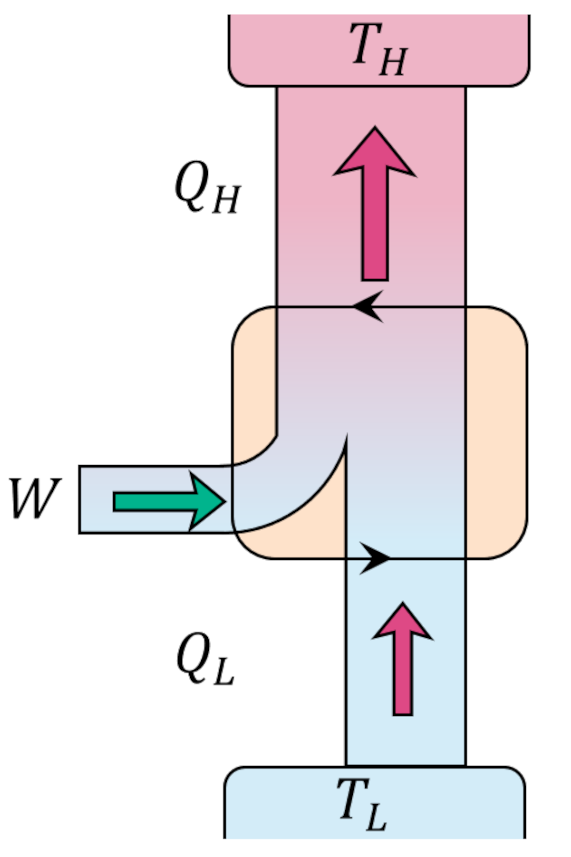
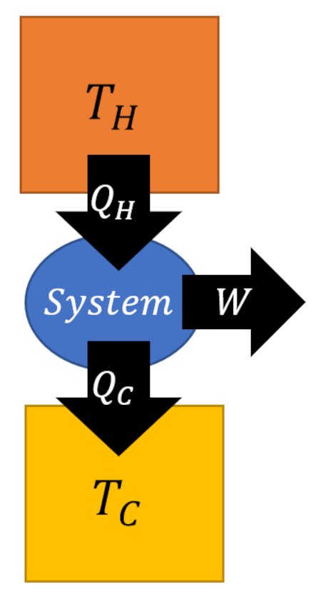
In its interaction with the system, the surroundings either absorbs or supplies some heat $Q_{sur}$ to the system such that $Q_{sys} = – Q_{sur}$.  If the surroundings constitute a reservoir such that $T$ is constant (i.e., a heat bath) the change in entropy of the surroundings can be expressed as

\[ \Delta S_{sur} = \frac{Q_{sur}}{T} =  – \frac{Q_{sys}}{T} \; .\]

With this result, we can now write the total change in the entropy of the universe without referencing anything more than the system (even the temperature, since constant, is measured in the system):

\[ \Delta S_{uni} = \Delta S_{sys} – \frac{Q_{sys}}{T} \; .\]

At this point, we’ve eliminated any need to refer to the surroundings and we can drop the ‘sys’ subscript in everything that follows. 

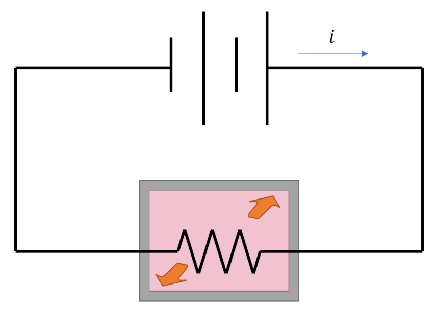
Now if the surroundings also confine the system to a constant volume $V$ (e.g., the process takes place in a pressure cooker), we know that the work performed by the system is identically zero and by the first law

\[ \Delta U = Q_{sys} \; . \]

Combining the previous two results we get that the total entropy of the universe can be expressed as

\[ \Delta S_{uni} = \Delta S_{sys} – \frac{\Delta U}{T} \; .\]

Next, we use the Helmholtz free energy

\[ F = U – TS \; .\]

as an auxiliary function for the system whose differential is

\[ dF = dU – dT S – T dS = dU- T dS \; , \]

where we used the constant temperature assumption to set $dT = 0$.  Everything in this relationship can also be expressed in terms of finite changes since every term in the expression is a state variable.  Now we can combine this expression with the expression relating the total entropy of the universe to the system to get

\[ \Delta F = T \Delta S – T \Delta S_{uni} – T \Delta S = -T \Delta S_{uni} \; . \]

Since $\Delta S_{uni} > 0$ must be satisfied for spontaneity, we see (after some simple rearranging) that the criterion of spontaneity for processes that take place at a constant temperature and volume is

\[ \Delta F < 0 \; \]

with no reference to anything outside the system or process of interest.

The value of the Helmholtz free energy, which is often called the Helmholtz potential and is sometimes denoted by $A$ (from the German word arbeit, which means work), represents that fraction of the store of internal energy that is available to do work.

Alternatively, if the surroundings provide a constant pressure (e.g., the process takes place in a vessel open to the atmosphere), we can use the Gibbs free energy for the system

\[ G = U + PV – TS \; .\]

This case is slightly more complicated and it helps to use the definition of enthalpy $H = U + PV $ since doing so allows us to relate the system heat at constant pressure to the change in enthalpy as follows.

Take the differential/delta of the enthalpy to get

\[ \Delta H = \Delta U + P \Delta V = Q_{sys} – W + P \Delta V \; . \]

Assuming the system work in entirely mechanical expansion/compression work (i.e., $PV$ work) gives

\[ \Delta H = Q_{sys} \; .\]

This result leads to a similar equation for total entropy change

\[ \Delta S_{uni} = \Delta S_{sys} – \frac{\Delta H}{T} \; . \]

We then take the differential/delta of the Gibbs free energy

\[ \Delta G – \Delta H – T \Delta S_{sys} \; \]

and then eliminate the enthalpy change in favor of the change in the total entropy to get the criterion for spontaneous processes at constant temperature and pressure

\[ \Delta G < 0 \; .\]

The value of the Gibbs free energy, which is often called the Gibbs potential, represents that fraction of the store of internal energy that is available to do non-mechanical work.

At this point we can pause and take stock of what we did.  We were able to achieve White’s vision (which, of course he achieved himself) by eliminating any notion of the universe and total entropy by the use of the Helmholtz or Gibbs free energies and by using a mixed version of the first law where heat and work lived side-by-side with the state variables.  This movement between different perspectives is what makes thermodynamics so thorny for the beginning student and this discussion is particularly instructive as a result.  The remaining questions about the different types of work (non-mechanical versus mechanical) will have to wait until a future blog.

Up to this point, the discussion of entropy woven throughout the last many columns have featured entropy as a phenomenological parameter derived from the various equivalent formulations of the second law and clever, inventive ways of decomposing cyclical processes using the reversible steps of the Carnot cycle.  In this post, it is worth taking a breather from all the abstract theory by looking at a particularly instructive problem that has been used in a variety of pedagogical contexts: the situation of supercooled water.  This problem illustrates the thinking that a classical thermodynamicist (i.e. someone who is not using the molecular interpretation) would use.  The precise wording that we’ll follow is taken  from problem 20.21 of the Fundamentals of Physics, 10^th Edition – Halliday & Resnick, Walker, which reads:

This problem is interesting because the sudden and irreversible (to be verified later) transition of the water from a liquid drop to solid shard is not representable as a well-defined sequence of equilibrium states.  Nonetheless, we can calculate the change in entropy by imagining a reversible process that connects the initial state (supercooled drop) to the final state (frozen shard) as being made up of three legs.  By analyzing the changes along each reversible leg, we can arrive at the total change of the entropy and then, by relying on the fact that everything is now expressed in terms of state variables, we can let go of any appeal to reversibility.  Effectively, this three-legged process is a scaffold that can be thrown away once the underlying structure has been erected and the change in entropy obtained.    

In the first leg we reversibly heat the drop from its supercooled temperature ($T_C = 268 K$) until it is at its freezing point ($T_H = 273 K$).  On the second leg, we allow the drop to freeze naturally and reversibly into a shard of ice.  In the third leg, we finally cool the shard of ice back down to the $T_C$.  

For the first and third legs, we can relate the change in temperature $dT$ to the quantity of heat ${\tilde d}Q$ exchanged between the water (the system) and the surrounding air (the environment) as

\[{\tilde d}Q = m \, c \, dT \; ,\]

where $c$ is the specific heat capacity, which is assumed, for simplicity, to be constant over the temperature range, depending only on the phase of the material, and $m$ is the mass of the water. For water, the specific heat in liquid form is cited by the text as $c_L = 4.19 J/gK$ and the specific heat in solid form is $c_S = 2.22 J/gK$. 

For the second leg, we use the standard definition of the latent heat of fusion, $L_F$ to tell us that the heat shed to the environment is

\[ {\tilde d}Q_{freeze} = -L_F m \; ; \]

for water $L_F = 333 J/g$. Note that the sign is negative since heat moves out of the drop to the environment.

The changes in entropy along legs one and three are:

\[ \Delta S_{leg_1} = \int_{T_C}^{T_H} \frac{{\tilde d}Q}{T} = \int_{T_C}^{T_H} \frac{m c_L dT}{T} = m c_L \ln \left( \frac{T_H}{T_C} \right) \; \]

and

\[ \Delta S_{leg_3} = \int_{T_C}^{T_H} \frac{{\tilde d}Q}{T} = \int_{T_C}^{T_H} \frac{m c_S dT}{T} = – m c_S \ln \left( \frac{T_H}{T_C} \right) \; . \]

The change in entropy along leg two (reversible freezing at $T_H$) is

\[ \Delta S_{leg_2} = – \frac{{\tilde d}Q}{T_H} = \frac{L_F m}{T_H} \; . \]

Combining leads to a total change in entropy of the drop  

\[ \Delta S_{drop} = m ( c_L – c_S ) \ln \left( \frac{T_H}{T_L} \right) – \frac{L_F m}{T_H} \; .\]

Since the drop freezes suddenly and irreversibly, one might think that the $\Delta S$ should be positive but this conclusion ignores the fact that the second law only says that the total, universal entropy change should be positive for an irreversible process.  The numerical computation is

\[ \Delta S = 1g (4.19-2.22) J/gK \ln(273/268) + \frac{333 J/g \cdot 1 g}{273 K} = -1.18 J/K \; .\]

Our faith in thermodynamics will be bolstered if we can show that the total entropy has increased.  The change in the entropy of the surroundings is given by

\[ \Delta S_{sur} = \frac{{\tilde d}Q_2}{T_L}  = \frac{ L_F m}{T_L} \; . \]

Note that this expression is almost identical to that used in leg 2 of the reversible process with the single change that the heat is delivered to the environment at the lower temperature $T_L$ instead of the higher one. 

The total change in the entropy of the universe is

\[ \Delta S_{uni} = \Delta S_{drop} + \Delta S_{sur} = m ( c_L – c_S ) \ln \left( \frac{T_H}{T_L} \right) + L_F m \left( \frac{1}{T_L} – \frac{1}{T_H} \right) \; .\]

Putting numbers to it gives

\[ \Delta S_{uni} = -1.18 J/K + \frac{333 J/g \cdot 1 g}{268 K} = -1.18 J/K + 1.24 J/K \\ = 0.059 J/K > 0 \; .\]

The fact that the overall universal entropy increases rigorously what we already expected from the framing of the problem – that the sudden freezing of the supercooled drop is an irreversible process. Finally, it is worth noting two points that follow from the observation that $c_L > c_S$ for water and $T_L < T_H$, by definition for supercooling.  First, the naïve model developed here suggests that water can be supercooled to any temperature since $\Delta S_{uni}$ is always positive.  Clearly water is more subtle in its behavior as evidenced by the fact that there is an observed lower limit ($-48^{\circ} C$) below which supercooled water cannot exist.   Second, isn’t at all clear that the heat capacity of an arbitrary material in a liquid phase should always be greater than that in its solid phase, although basic considerations of statistical mechanics suggests that it should be.

The last post derived the Clausius inequality

\[ \oint \frac{{\tilde d} Q}{T} \leq 0 \; , \]

using a rather subtle and clever technique (presented by Fermi in his book Thermodynamics without further attribution, although it is certain that the argument dates back probably more than fifty years earlier) in which a complex cyclical process was augmented with a set of Carnot cycles that interacted with the original reservoirs and an external heat reservoir called the base.  By encapsulating the original cycle and these auxiliary Carnot cycles as a single, black box engine and then invoking Kelvin’s postulate on their total interaction with the base, we were able to arrive at the expression above, with the equality holding only in the limiting case that the original cycle was reversible. 

Since an earlier post demonstrated that Kelvin’s and Clausius’s postulates (both of which essentially say that perpetual motion is impossible) were different facets of the second law and Kelvin’s postulate is used to derive the Clausius inequality, it is clear the inequality is yet another expression of the second law.  The advantage of this third way of expressing the second law is that, as a mathematical expression, it motivated the definition of entropy, which has dominated the conversation ever after.  The quantitative nature of the definition of entropy allows for two useful innovations: 1) the numerical determination for whether a process is allowed or disallowed to proceed spontaneously and 2) and rewriting of the first law in terms of $S$ since it is a state variable.  Let’s deal with each in turn.

By definition, spontaneous processes occur naturally in a single direction; heat flows from a warmer body to a colder one; some chemical reactions run only in one direction, eggs that fall on the ground break never to reassemble themselves; and so on.  Running movies of these processes backwards looks unnatural even though movies of billiard ball collisions and the motion of celestial objects do.  None of these spontaneous processes are forbidden by energy conservation, they simply don’t happen.  As Carter points out in his book Classical and Statistical Thermodynamics, the first law is general, useful, and simple but is ultimately unsatisfactory since it doesn’t distinguish between allowed and disallowed processes. 

Obviously, spontaneous process are irreversible even if the precise logical connection between these two terms is not completely established.  For example, if the converse is true then we can also conclude that all irreversible processes are spontaneous.  This kind of question is more subtle that it might seem at first glance.  We will have to content ourselves with looking at irreversible processes since irreversibility takes mathematical expression within the Clausius inequality. 

To determine if a process is irreversible, one simply calculates the entropy change $\Delta S$ between the before and after states.  If the change in entropy is positive, the process is irreversible and we conclude it will happen spontaneously in nature.  Note that the specific path by which the final state is reached from the initial state is irrelevant since entropy is a state variable.  Heat need not flow from a hotter to colder body in exactly the same way every time the same experiment is run for us to conclude that the process will operate irreversibly.  This is the power of defining entropy as an exact differential (i.e., state variable) and using the change as the indicator.

To understand this further, we follow the example from Section 6.5 of Carter (which itself follows Fermi’s presentation in Sec. 13) where we imagine an irreversible process that transitions a system between two thermodynamic states $a \rightarrow b$ and a reversible process that carries the system back. 

By the Clausius inequality

\[ \int_a^b \frac{ {\tilde d} Q}{T} + \int_b^a \frac{dQ_r}{T} \leq 0 \; . \]

Reversing the limits of the second integral (the reversible process) and rewriting the inequality gives

\[ \int_a^b \frac{{\tilde d} Q}{T} \leq \int_a^b \frac{dQ_r}{T}  \; . \]

The reversible integral can be immediately written as the difference between the entropy values at the two states giving a final relation

\[ \Delta S = S_b – S_a \geq \int_a^b \frac{{\tilde d} Q}{T} \; \]

Now if the system is isolated, then $d\tilde Q = 0$, and we have that $\Delta S \geq 0$.  This observation is the origin of the law that the entropy of the universe must always be increasing.

On a more modest scale, a nice simple example of the power of this method comes from General Chemistry, The Essential Concepts by Chang and Overby.  In Example 18.2, they ask the student, using standard entropy values, to calculate the entropy change in two chemical reactions at $25 C$.

In the first chemical reaction

\[ CaCO_3(s) \rightarrow CaO(s) + CO_2(g) \; \]

has an entropy change of

\[ \Delta S^{\circ} = S^{\circ}(CaO) + S^{\circ}(CO_2) – S^{\circ}(CaCO_3)\\ = (39.8 + 213.6 – 92.9) J/(K \cdot mol) = 160.5 J/(K mol) \; , \]

while in the second chemical reaction

\[ N_2(g) + 3H_2(g) \rightarrow 2NH_3(g) \; \]

has an entropy change of

\[ \Delta S^{\circ} = 2 S^{\circ}(NH_3) – S^{\circ}(N_2) – 3 S^{\circ}(H_2)\\= (2 \cdot 193 – 192 – 3 \cdot 131) J/(K \cdot mol) = -199.0  J/(K mol) \; . \]

From these values, we would expect the first chemical reaction to occur spontaneously while the second would not. 

The second innovation that entropy as an exact differential (i.e., state variable) provides is an incredibly useful rewrite of the first law of thermodynamics.  The initial expression for the change in internal energy $U$ was expressed in terms of vague ‘inexact’ differentials as

\[ dU = {\tilde d} Q – \tilde{d}W \; ,\]

where, ${\tilde d} Q$ is the heat (positive if it flows into the system) and $\tilde{d}W$ is the work (positive if the system performs is).  We needed to specifically account for heat flow and work performed at each and every step in the process, a nearly impossible task for reversible processes and almost certainly an impossible one for irreversible processes.

The introduction of the entropy provides the far more useful expression

\[ dU = TdS – PdV \; ,\]

where every term on the right-hand side is a state variable.  This change is more than cosmetic as having only state variables frees us from having to pay attention to how a system evolves and allows us to focus only on the before and after conditions which is a far easier task.

To appreciate how this rewrite is possible, we follow the argument in Carter’s Section 6.8.  Carter starts by noting that the Clausius inequality allows us to conclude that

\[ dS \geq \frac{ {\tilde d} Q}{T} \; . \]

The inequality can be removed by accounting for reversible and irreversible pieces separately so that

\[ TdS \equiv dQ_r = {\tilde d} Q + \epsilon \; , \]

where $\epsilon$ is some positive quantity and the $r$ subscript on $dQ_r$ reminds us that that is the quantity of heat into/out of the system during the reversible process.  Substituting this into the first law gives

\[ dU = TdS – \epsilon – {\tilde d} W = T dS – ({\tilde d} W + \epsilon) \; .\]

The quantity in the parentheses is the amount of useful work done by the system plus the ‘tax’ associated with the system having to overcome dissipative forces.  It is precisely the pressure work $PdV$ done by the system and so we arrive at

\[ dU = TdS – PdV \; .\]

without any loss of generality. 

Over the past three posts, we’ve laid the groundwork for the mathematical formulation of entropy.  The logic started with two separate but equivalent formulations of the second law:  Kelvin’s postulate and Clausius’ postulate.  Both postulates summarize some aspect of those processes that never occur even though the first law (conservation of energy) doesn’t forbid them.  The Kelvin postulate says that we can never use a cyclic process to convert any energy extracted as heat from a reservoir into work.  Likewise, the Clausius postulate says that we can’t use a cyclic process to make energy flow from a colder system to a warmer one without expending some energy in the form of work during the process.  The Carnot cycle is integral in proving that these two postulates are different facets of the same second law, which colloquially has often been characterized as saying that there is no such thing as a free lunch.

The Carnot cycle has additional responsibilities as a central player in our thermodynamic drama.  It’s reversible legs of adiabatic expansion and compression punctuated by isothermal counterparts sets a limit on the efficiency of any engine (Kelvin) or refrigerator (Clausius).  So, it shouldn’t be a surprise that it still has additional roles it needs to play.  One such role, which was touched on in the post entitled Carnot Cycle, is as the basic ‘atom’ that can used to decompose more complicated cycles.

We are going to use this property to prove two things: 1) the Clausius inequality that further defines the role that entropy plays in descriptions of the second law and 2) that entropy is a state variable. 

The arguments presented here closely follow those found in Enrico Fermi’s Thermodynamics supplemented with ideas from Ashley Carter’s Classical and Statistical Thermodynamics.

We start by imaging a cyclic process in which a system interacts with $N$ thermal reservoirs at temperatures $T_1, T_2, \ldots, T_N$.  In some of these interactions the system’s temperature $T_S$, which varies throughout the cycle, will be higher than the reservoir temperature and the system will deliver heat in the amount $Q_i$ to the reservoir. In others, $T_S < T_i$ and the system will absorb heat in the amount $Q_i$ from the reservoir.  The quantities $Q_i$ will be negative when the energy flows out of the system and positive when energy flows in.

The Carnot decomposition begins by imaging another thermal reservoir, called the base, with temperature $T_0$, which, without loss of generality, is taken to higher than any other temperature in the problem.  At each stage of the system cycle, we place a Carnot cycle into contact with the $i^{th}$ reservoir and the base.  If the system absorbs heat from the $i^{th}$ reservoir we run the Carnot cycle as an engine extracting work $W_i$ from the energy transfer from the base to the $i^{th}$ reservoir.  The following figure shows an example of this type of interaction.

When the system delivers heat to the $i^{th}$ reservoir we run the Carnot cycle as a refrigerator consuming some work $W_i$ to extract the same amount of heat from the reservoir and dump it (and excess heat) into the base.

The following animation shows three turns through what we dub the Fermi Cycle in which our system interacts with 6 reservoirs.  Blue-shaded reservoirs have temperatures lower than the system temperature at the time of the interaction while yellow-shaded ones have higher temperatures.

By coupling a Carnot cycle to each stage of the interaction, we can relate the heat absorbed or delivered by the system to the heat exchanged between the base and the various reservoirs by

\[ Q_{0,i} = -\frac{T_0}{T_i} Q_i \; ,\]

which is just a relabeling of a relation

\[ \frac{Q_H}{T_H}  = \frac{-Q_L}{T_L} \; ,\]

derived in the previous post.

The total heat transferred from the base is

\[ Q_0 = \sum_{i=1}^N -\frac{T_0}{T_i} Q_i = – T_0 \sum_{i=1}^N \frac{Q_i}{T_i} \; . \]

Despite the overall minus sign, it isn’t immediately clear whether $Q_0$ is positive, negative, or zero since the $Q_i$’s can be of any sign.  This ambiguity dissolves when we realize that in a full turn through the Fermi cycle, the original system, the helper Carnot cycles, and the individual reservoirs, which collectively can be taken as a ‘black box’ engine, in and of itself, have returned to its initial state.  By the first law, the change in this black box’s internal energy is zero and so the heat exchanged (in or out) has to be equal to the work performed (done by or done to) by the base.  By Kelvin’s postulate, it is impossible to extract work from the base so the work has to be zero or negative and so we conclude that $Q_0$ is zero and negative as well, leading us to Clausius’ inequality

\[ \sum_{i} \frac{Q_i}{T_i} \leq 0 \; .\]

Before pushing this expression farther, it is instructive to reflect on the physical content of the previous argument.  The fact that the work is negative in a complex irreversible engine reflects the engine’s need for a power source to run and the fact that the heat is also negative (since $Q=W$) reflects that such an engine creates heat that it dumps to the environment as a byproduct.  Each automobile engine testifies to this. 

Only when the engine is truly reversible can we get equality with zero.  This is seen from the fact that if the process is reversible then, upon running the cycle in the opposite direction, all the heat values become negative and so the heat moved from the based in the reversed process is

\[ Q_{0,r} = – T_0 \sum{i} \frac{-Q_i}{T_i} = T_0 \sum_{i} \frac{Q_i}{T_i} = – Q_0 \; .\]

But $Q_{0,r}$ must also obey the Clausius inequality and we conclude $Q_{0,r} = Q_{0} = 0$.

While Clausius’ inequality was derived for a discrete set of reservoirs we can imagine transitioning to a continuum as the number is increased without bound but with each exchange shrinking in size.  We ‘loosely’ summarize this as

\[ \oint \frac{{\tilde d} Q}{T} \leq 0  \leftrightarrow \sum_{i} \frac{Q_i}{T_i} \leq 0 \; , \]

where the equality is satisfied for reversible processes. Note that the reasons for the tilde on the $d$ within the integral are due to the fact that the heat is not an exact differential.

The final point to note is define the differential entropy of a system as

\[ dS \equiv \frac{{\tilde d} Q}{T} \; .\]

So defined, the entropy is a state variable since any two states, visualized, for example, as points in the $p-V$ can have a value for the change $\Delta S$ unambiguously defined for any reversible process connecting them.  The entropy is path independent, otherwise a trip through the cycle would result in zero, and thus, is an exact differential. 

Up to this point in this classical survey of entropy, the star player, namely entropy itself has remained unseen but perhaps felt or anticipated.  In this post, we actually get to the definition of entropy from the phenomenological point of view that is equilibrium thermodynamics. 

To recap, we’ve covered the following points.  To begin, the first law of thermodynamics neither restricts the types of allowed energy transformations nor the direction, order, or frequency.  Like a good accountant working with double entry bookkeeping, the first law merely insists that the books balance and that energy losses from one account are balanced with gains in others – in short that energy is conserved.  Next, we have the postulates of Clausius and Kelvin, which, much like financial regulators, place (or at least assert that nature places) restrictions on the types of allowed transactions.  These restrictions naturally led to the notion of energy transfers falling into two broad categories: reversable and irreversible.  Third, we find that the Carnot engine, with is incredibly simple set of 4 reversible processes, provides profoundly universal conclusions including the facts that the Kelvin and Clausius postulates each logically imply the other and that both are just two of many different facets of the larger second law of thermodynamics (although we stopped short of stating this in no uncertain terms since we hadn’t yet defined classical entropy).  Finally, we established that no engine in the world can match the efficiency of the Carnot engine which is given by

\[ \epsilon_{Carnot} = 1 – \frac{|Q_H|}{|Q_L|} \; , \]

where $|Q_H|$ and $|Q_L|$ are the amounts of heat extracted from and dumped to the high ($T_H$) and low ($T_L$) temperature reservoirs, respectively.  This implies that irreversibility is tied to the limitations found within the second law but this expression is hard to use since the amount of heat moved into or out during the cycle depends on the nature of the working substance.

To see this connection more clearly, let’s return to the Carnot engine but this time specifying the working substance to be an ideal gas with the familiar equation of state

\[ P V = n R T \; , \]

which we will use on each leg of the Carnot cycle, shown below.

As a reminder, we are using the Clausius sign convention that assigns positive values to heat that flows into the ideal gas (system for short) and to work done by the system on its surroundings so that the first law reads $\Delta U = Q – W$.  The pair of points ${\mathcal A}$ and ${\mathcal B}$ and the pair ${\mathcal C}$ and ${\mathcal D}$ are connected by isotherms.  We’ll take, as given, the well-known result that the internal energy of an ideal gas depends only on temperature so along these isotherms $\Delta U_{{\mathcal A} \rightarrow {\mathcal B}} = 0 $ and $\Delta U_{{\mathcal C} \rightarrow {\mathcal D}} = 0$.  From the first law, the constancy of the internal energy means that the heat that enters or exits the system is identically equal to the work:  $Q_H = -W_{{\mathcal A} \rightarrow {\mathcal B}}$ and $Q_L = -W_{{\mathcal C} \rightarrow {\mathcal D}}$.  Each of these works can be calculated easily by relating the pressure work $dW = P dV$ to the equation of state.

For the isothermal expansion

\[ Q_H = -W_{{\mathcal A} \rightarrow {\mathcal B}} = \int_{{\mathcal A}}^{{\mathcal B}} P d V \; .\]

Solving the equation of state for the pressure, substituting that result into the integral to eliminate $P$ and pulling out the constant temperature $T_H$ gives

\[ Q_H  =  n R T_H \int_{{\mathcal A}}^{{\mathcal B}} \frac{d V}{V} = n R T_H \ln \left( \frac{V_{{\mathcal B}}}{ V_{{\mathcal A}}}\right)\; .\]

As a check, note that since $V_{{\mathcal B}} > V_{{\mathcal A}}$ the heat transferred between the system and the higher temperature reservoir is positive ($Q_H > 0$) and that the work is negative ($W < 0$) since the system ‘pushes on’ the surrounding as it expands, both of which are consistent with the Clausius sign convention.

A similar analysis for the isothermal compression gives

\[ Q_L =  n R T_L \ln \left( \frac{V_{{\mathcal D}}}{ V_{{\mathcal C}}}\right)\; .\]

As additional check, note that since $V_{{\mathcal D}} < V_{{\mathcal C}}$, that the heat transferred between the system and the lower temperature reservoir is negative ($Q_L$) representing heat flowing out, as expected.

We can now eliminate the volumes at each end state from these expressions for the heat flows by relating $T$ and $V$ on the adibats.  The heat flow, by definition, is zero on these processes meaning that $\delta U = – W$.  We will also assume that the ideal gas is calorically perfect so that the heat capacity at constant volume $C_V$ is a constant so that internal energy, which only depends on temperature, can be expressed as

\[ d U = n C_V d T \; . \]

Setting this expression equal to the work $dW = – P dV$ and eliminating the pressure using the equation of state gives

\[ C_V dT = -\frac{R T}{V} dV \; , \]

which can be immediately integrated from initial to final values to give

\[ \frac{T_f}{T_i} = \left( \frac{V_f}{V_i}\right)^{-\frac{R}{C_V}} = \left( \frac{V_f}{V_i}\right)^{1- \gamma}\; , \]

where the ratio $R/C_V$ is replaced with $\gamma – 1$ to match the usual convention.  Finally, cross-multiplication to gather initial and final values on the left- and right-hand sides, respectively, yields

\[  T_i V_i^{\gamma – 1} = T_f V_f^{\gamma – 1} \;. \]

Applying this formula to the adiabatic expansion from ${\mathcal B} \rightarrow {\mathcal C}$ and the adiabatic compression from ${\mathcal D} \rightarrow {\mathcal A}$ gives

\[ T_H V_{{\mathcal B}}^{\gamma – 1} = T_L V_{{\mathcal C}}^{\gamma – 1} \; \]

and

\[ T_H V_{{\mathcal A}}^{\gamma – 1} = T_L V_{{\mathcal D}}^{\gamma – 1} \; .\]

Dividing the previous equation by the last one gives

\[ \frac{ T_H V_{{\mathcal B}}^{\gamma – 1}}{ T_H V_{{\mathcal A}}^{\gamma – 1}} = \frac{ T_L V_{{\mathcal C}}^{\gamma – 1}}{ T_L V_{{\mathcal D}}^{\gamma – 1}} \; ,\]

which simplifies to

\[ \frac{V_{{\mathcal B}}}{V_{{\mathcal A}}} = \frac{ V_{{\mathcal C}}}{ V_{{\mathcal D}}} \; .\]

These ratios enable us to eliminate the volumes from the computations of heat obtained from analyzing the isothermal steps leaving us with

\[ \frac{Q_H}{T_H}  = \frac{-Q_L}{T_L} \; ,\]

where ‘extra’ minus sign come from flipping $V_{{\mathcal D}}/V_{{\mathcal C}}$ in the original expression to $V_{{\mathcal C}}/V_{{\mathcal D}}$.  The question of sign convention can be totally eliminated by with absolute values to

\[ \frac{|Q_H|}{T_H}  = \frac{|Q_L|}{T_L} \; .\]

The simplicity of this expression belies it profundity.  Despite all the state changes in the Carnot cycle the ratio of the heat transferred between the system and the higher temperature reservoir to its temperature is equation to the ratio of the heat transferred between the system and the lower temperature reservoir and its corresponding temperature.  This ‘conservation’ of ‘whatever’ lead us to propose a new quantity denoted by $S$ which says

\[ S \equiv \frac{Q}{T} \; .\]

And, thus, entropy has entered onto the stage of thermodynamics.

Before we go, it is worth noting the point Carter raises in his book Classical and Statistical Thermodynamics, that entropy so defined complements the conjugate nature of pressure and volume.  Pressure is an intensive variable that when multiplied by the extensive variable volume leaves a quantity (i.e., work) with units of energy.  Temperature is an intensive variable that when multiplied by entropy also leaves a quantity (i.e., heat) with units of energy.  In this way, entropy perhaps could have been anticipated without the analysis from above.

We’ll explore this classical definition of entropy more deeply in the next post, including showing that it is a state variable and fleshing out some of its connections to irreversibility.

In the last post, we explored Kelvin’s and Clausius’ postulates and found that each of them, in their own way, put limits on the way in which energy could be exchanged in physical systems.  We also showed that each of them logically implied the other thereby demonstrating that both were two separate facets of the second law and that a particular result of the Carnot cycle was an integral part of the proof.  Now it is time to take a much deeper look at the Carnot cycle and the preeminent place it holds in understanding entropy.  Several of the arguments presented here closely mirror those in Carter’s Classical and Statistical Thermodynamics and several of the figures and the argument about the efficiency of the Carnot cycle were inspired by the Fundamentals of Physics by Halliday, Resnick, and Walker.

The Carnot cycle is a special kind of engine or refrigerator depending on how it is run.  For clarity, we define engines and refrigerators as machines that execute a set of thermodynamic processes on a physical system, called the working substance, that result in some in the transfer of energy, either in the form or work or heat, but which return the working substance to its initial state.  Taken together, the set of processes is called a cycle.

Any thermodynamic process connects an initial state ${\mathcal A}$ to a terminal state ${\mathcal B}$ through a locus of intermediate thermodynamic states.  Thermodynamic processes fall into one of two broad categories: reversible and irreversible, with the key difference being that reversible processes naturally run from in the opposite direction (${\mathcal B}$ to ${\mathcal A}$) while irreversible processes do not (hence their names).  An example of a reversible process in which energy is exchanged is an elastic collision between two balls.  A movie of the collision looks physically reasonable whether it is run forwards or backwards.  An example of an irreversible process is the heating of a tank of water by a resistor (of resistance $R$) powered by a battery delivering a current $i$.  The heat delivered to the tank during some time span $\Delta t$ is $Q = {\mathcal P} \Delta t = i^2 R \Delta t$.  That amount of heat raises the temperature of the tank at the expense of depleting an equal amount of stored energy in the battery.  This process looks natural but none of us would expect that we could recharge the battery simply by cooling the tank back to original temperature.  This one-way character of irreversible processes gives the physical world the ‘arrow of time’ and many consider it to be one of the hallmarks of entropy.

What makes the Carnot cycle so special is that it represents an ideal engine that operates between two heat reservoirs in which all the processes are reversible.  It consists of four steps: ${\mathcal A} \rightarrow {\mathcal B} \rightarrow {\mathcal C} \rightarrow {\mathcal D} \rightarrow {\mathcal A}$. 

In the first step (${\mathcal A} \rightarrow {\mathcal B}$) the working substance absorbs $Q_H$ from the high temperature reservoir such that it isothermally expands and performs positive work.  In the second step (${\mathcal B} \rightarrow {\mathcal C}$) the working substance expands adiabatically ($Q=0$) while it also does positive work.  The third step (${\mathcal C} \rightarrow {\mathcal D}$) consists of the working substance being isothermally compressed by dumping $Q_L$ to the cold temperature reservoir will having work done on it (i.e., negative work is done by the system).  In the fourth step (${\mathcal D} \rightarrow {\mathcal A}$), the working substance is returned to its initial state by being adiabatically compressed.

Theorists usually represent the Carnot cycle visually as a set of curves plotted in the pressure-volume ($PV$) plane.

We typically imagine the working substance as an ideal gas.  In this case, the abstract steps of the Carnot cycle become familiar processes in terms of the usual cylinder-and-piston arrangement.

Since the change in internal energy of the system must be zero (the gas ends in the same state that it started in), the first law tells us that the work delivered by the engine $W = |Q_H| – |Q_C|$.  Standard practice is to visualize an engine (executing the Carnot cycle or otherwise) abstractly as an systems of interacting boxes that take in and dump heat of quantities $Q_H$ and $Q_L$, respectively, in the process delivering work of amount $W$.

The efficiency of the engine is the fraction of the heat energy that enters the engine that results in useful work and is given by

\[ \epsilon = \frac{W}{|Q_H|} = 1 – \frac{|Q_C|}{|Q_H|} \; . \]

Since every process is reversible, the Carnot cycle can be operated in the opposite order giving a refrigerator that is able to move heat from the lower temperature reservoir to the higher temperature reservoir at the expense of work being provided to the cycle rather than being delivered.

We should now ask if there are any engines that can operate more efficiently than the Carnot cycle.  In the process of answering this question in the negative we will see more clearly the connections with Kelvin’s and Clausius’ postulates and will understand why the Carnot cycle has a preeminent position in the field of thermodynamics.

We start our answer by conjecturing that there exists an engine, call it Engine X, whose operating efficiency is better than the Carnot cycle,

\[ \epsilon_X > \epsilon_{Carnot} \; .\]

This assumption doesn’t mean that Engine X takes in the same amount of heat as the Carnot engine nor dumps the same amount but simply that it delivers a given amount of work $W$ as a larger fraction of whatever it takes in.  Thus, if the Engine X absorbs $Q’_H$ joules from the higher reservoir to deliver $W$ joules of work then

\[ \frac{|W|}{|Q’_H|} > \frac{|W|}{|Q_H|} \; . \]

This inequality simplifies to

\[ |Q_H| > |Q’_H| \; .\]

By the first law,

\[ |Q_H| – |Q_L| = |W| = |Q’_H| – |Q’_L| \; , \]

which can be rewritten as

\[ |Q_H| – |Q’_H| = |Q_L| – |Q’_L| \; .\]

From our previous analysis of the efficiency, the quantity on the left-hand side is positive and so must be the quantity on the right-hand.  By using the work delivered by Engine X to power a Carnot refrigerator

we can create a process whose only effect is to move heat from a colder reservoir to warmer one directly violating the Clausius postulate.  If we accept the Clausius postulate we must reject the idea that any engine can be more efficient than the Carnot engine.

Two points in conclusion are worth making.  First, we might have expected this outcome given the special nature of reversible processes.  Second, given the Carnot cycle’s position as the gold standard of thermodynamics it should come as no surprise that we can always decompose an arbitrary process

into Carnot subprocesses

whose internal adiabats cancel and whose efficiency and total energy exchange can be determined by adding the individual subprocesses together (credit to Carter for making this point so clearly).

Next month, we’ll recast the Carnot efficiency in light of using an ideal gas as the working substance and will begin to see the emergence of entropy.

This month we were return to our exploration of entropy after our brief detour into field theory.  The earlier posts explored the definition of entropy derived from the statistical mechanics. In this installment, we return to the thermodynamic roots of entropy that originated in the analysis of the 19^th Century. Our key players in this drama are Sadi Carnot, Lord Kelvin, and Rudolph Clasius, who will be with us both here and for several of the following posts.

This analysis closely follows the presentation found in Enrico Fermi’s book Thermodynamics with some additional extensions in the logic and new, explanatory diagrams that attempt to provide a cleaner approach to traditional material.

Thermodynamics rests upon the idea of a system in equilibrium so that we can characterize it in terms of a very small number of state variables compared with the overwhelmingly enormous number of degrees of freedom the system possesses.  A bottle of water is a good poster child for a system in equilibrium. The bottle can be described by the amount of water $m$ (or the number of moles $n$), the volume it occupies $V$, its temperature $T$, pressure $P$, and the like. Even if the water were not pure and we were forced to also specify the percentage of impurities by type there would still be far, far fewer numbers to specify than the incredibly astronomical number of position and velocity components required to describe the state as Newton would.  The state variables are completely independent of how the system made it into that configuration. Their values represent average quantities where individual, finer-grained fluctuations are smeared out.  There are two state variables that stand above the rest both in importance: the internal energy $U$ and the entropy $S$.

The internal energy is relatively familiar to us based on its analogy to the traditional energies defined in classical mechanics and electrodynamics.  That said, it took quite a long time before it was appreciated in the mid-1800s that mechanical energy and heat were equivalent.  When the dust had settled, the first law of thermodynamics had been postulated as

\[ \Delta U = Q – W \; , \]

where $Q$ is the heat that enters or leaves the system and $W$ the work done by the system on its surroundings.  The sign convention is such that heat entering and work performed are both positive quantities.  If one regards energy as the ‘currency’ for physical transactions, then the first law amounts to an accounting principle that says the books must balance and, in this regard, it is relatively easy to understand the physical content.

The entropy, on the other hand, is more difficult to summarize succinctly.  Many people can offer euphemisms stating that the principle of entropy means that there is ‘no free lunch’ or that it ‘forbids perpetual motion’ but these euphemisms don’t provide much in the way of physical understanding.

There are several steps in providing a firm understanding of entropy.  The rest of this post centers on the first step which involves the different ways of expressing the limitations the second law recognizes in the conversion between work and heat.

We start by looking at the isothermal expansion of an ideal gas, in which a flame provides the heat which causes the expantion.  Since the internal energy of an ideal gas only depends on temperature, as long as the temperature remains constant, there is no change in the internal energy $\Delta U = 0$.  Then from the first law $W = Q$, which means that all of heat energy is changed into the work needed to raise the piston.

It natural to ask if all physical processes allow for a complete conversion of heat to work as allowed by the first law whenever $\Delta U = 0$ or are there limitations on how efficient arbitrary physical processes can be? 

After much analysis and experimentation, most of which was done in the 1800s, the second law of thermodynamics emerged with a clear set of limitations for how changes between heat and work are made.  Its modern form expresses the statement in terms of entropy but we will avoid it in favor of more macroscopic statements.

Fermi provides two postulates that capture different aspects of the second law. The first postulate, attributed to Lord Kelvin, states that:

Graphically this forbidden process is represented on a $PVT$ diagram as follows.

The circular arc reminds us that the state of the system must remain unchanged at the end of the transformation. 

The second postulate, attributed to Clausius, states

The graphical representation of this forbidden process as follows.

Note that both postulates rule out as impossible certain transformations that leave the state of the system otherwise unchanged (“only final result is…”).  Since the state of system is unchanged we will focus on cyclic processes, of the kind used in engines, in which a complete circuit returns the system to its original state ($\Delta U = 0$) with some fraction of the heat absorbed being transformed into work.

The textbook example of a cyclic process is the Carnot cycle, which operates a system between two thermal reservoirs with temperatures $T_C$ and $T_H$ (with $T_C < T_H$). 

While the details of the Carnot cycle will be explored in the next post, for our purposes the final result relating the work derived to the heat exchanged given by

\[ W = Q_H – Q_C \; \]

will be all that is needed.

Fermi devotes a large amount of effort showing that the Kelvin and Clausius postulates are logically equivalent and are different facets of the same underlying limitations of the second law.

The first part of the proof, that Kelvin’s postulate implies the Clausius postulate, is the easiest to understand.  Suppose that the Kelvin postulate were false.  Then we could extract from system $A$ some work $W$ leaving system $A$ otherwise unchanged.  We then use the work to raise a block up an inclined plane gaining gravitational potential energy.  We then let the block slide down the plane using friction to transform the potential energy into heat which we can then dump to the hot reservoir in system $B$, thus violating the Clausius postulate.

The converse leg of the proof, that the Clausius postulate implies the Kelvin postulate, is a bit more difficult.  Suppose that the Clausius postulate were false and that it were possible to transfer some heat $Q_H$ from the cold reservoir at temperature $T_C$ with no other changes in the system to the hot reservoir $Q_H$.  As long as the amount of heat is consistent with what is normally adsorbed from by a Carnot cycle to produce an amount of work $W$ we then find that we can return the hot reservoir to its original state with no additional changes.  We could then use the Carnot cycle to adsorb this heat to produce some work $W$ thus extracting heat from the hot reservoir without any additional changes in violation of the Kelvin postulate.

The logical equivalence of the Kelvin and Clausius postulates demonstrate that these various limitations are different facets of the second law.  This logical structure serves as the launching pad for exploring the concept of entropy from the macroscopic point-of-view.

[Note added after publication – the equivalence between the Kelvin and Clausius postulates is nicely described here.]

The last post introduced the curvilinear mantra for students working with field equations in such disciplines as fluid mechanics, general relativity, and electricity and magnetism.  The textbook example (see, e.g. Acheson Appendix A, pp 352-3) is Euler’s equations for ideal fluids in two spatial dimensions. 

In cartesian coordinates these equations read

\[ \rho \left( V_x \partial_x + V_y \partial_y + \partial_t \right) V_x = – \partial_x p + f_x \;  \]

and

\[ \rho \left( V_x \partial_x + V_y \partial_y + \partial_t \right) V_y = -\partial_y p + f_y \; ,\]

whereas, in polar coordinates these equations read

\[ \rho \left( V_r \partial_r + \frac{V_\theta}{r} \partial_\theta  + \partial_t \right) V_r – \rho \frac{{V_\theta}^2}{r} = -\partial_r p + f_r \; \]

and

\[ \rho \left( V_r \partial_r + \frac{V_\theta}{r} \partial_\theta  + \partial_t \right) V_\theta + \rho \frac{V_r V_\theta}{r} = -\frac{1}{r} \partial_\theta p + f_\theta \; . \]

As discussed in the previous post, beginning students are often confused by two changes when transitioning from cartesian to polar coordinates.  The first is the appearance of $1/r$ scale factors that decorate various terms such as $V_\theta/r \partial_\theta$.  The second is the appearance of additional additive terms, such as $V_r V_\theta/r$. 

The curvilinear mantra explains these changes as follows: the scale factors come from minding the units and the additive terms show up to account for how the basis unit vectors change from place to place.

The first half of the mantra was covered in the previous post.  This post finishes the exploration by demonstrating how the additive terms arise due to the spatial variations of the basis vectors. 

The first step involves writing the position vector in terms of the polar coordinates and the cartesian unit basis vectors

\[ {\vec r} = r \cos \theta {\hat x} + r \sin \theta {\hat y} \; .\]

The polar unit basis vectors are defined by taking the derivatives of the position vector with respect to the polar coordinates and then unitizing.  The radial basis vector (not unitized) is

\[ {\vec e}_r \equiv \frac{\partial {\vec r}}{\partial r} = \cos \theta {\hat x} + \sin \theta {\hat y} \; .\]

Conveniently, this vector has a unit length and we can immediately write the radial unit basis vector as

\[ {\hat r} = \cos \theta {\hat x} + \sin \theta {\hat y} \; . \]

Following the same procedure, the polar angle basis vector (not unitized) is

\[ {\vec e}_\theta \equiv \frac{\partial {\vec r}}{\partial \theta} = -r \sin \theta {\hat x} + r \cos \theta {\hat y} \; . \]

This vector has length $r$ and so the polar angle unit base vector is

\[ {\hat \theta} = -\sin \theta {\hat x} + \cos \theta {\hat y}  \; .\]

Both vectors are independent of $r$ but do depend on $\theta$ and their variations are

\[ \partial_\theta {\hat r} = {\hat \theta} \; \]

and

\[ \partial_\theta {\hat \theta} = – {\hat r} \; . \]

At this point we have all the ingredients we need.  From the first part of the curvilinear mantra we have the velocity in polar coordinates is

\[ {\vec V} = V_r {\hat r} + \frac{V_\theta}{r} {\hat \theta} \;  \]

and the material (or total) time derivative is

\[ \frac{D}{Dt} = V_r \partial_r + \frac{V_\theta}{r} \partial_\theta + \partial_t \; , \]

where the scale factors on the polar angle terms are due to minding units.

Applying the material time derivative to the velocity gives

\[ \frac{D {\vec V}}{Dt} = \left( V_r \partial_r + \frac{V_\theta}{r} \partial_\theta + \partial_t \right) \left( V_r {\hat r} + \frac{V_\theta}{r} {\hat \theta} \right) \; . \]

Expanding this expression term-by-term yields

\[ V_r \partial_r \left( V_r {\hat r} \right) + \frac{V_\theta}{r} \partial_\theta \left( V_\theta {\hat \theta} \right) + \frac{V_\theta}{r} \partial_\theta \left( V_r {\hat r} \right) + \left(\partial_t V_r \right) {\hat r} + \left( \partial_t V_\theta \right) {\hat \theta} \; . \]

Expanding the derivatives, taking care to evaluate the spatial derivatives of the unit basis vectors, yields

\[ V_r \partial_r V_r {\hat r} + \frac{V_\theta}{r} \left( \partial_\theta V_\theta \right) {\hat \theta} – \frac{{V_\theta}^2}{r} {\hat r} + \left( \frac{V_\theta}{r} \partial_\theta V_r \right) {\hat r} + \\ \frac{V_\theta V_r}{r} {\hat \theta}  + \left(\partial_t V_r \right) {\hat r} + \left( \partial_t V_\theta \right) {\hat \theta} \; . \]

Collecting terms gives the radial term as

\[ V_r \partial_r V_r + \frac{V_\theta}{r} \partial_\theta V_r – \frac{{V_\theta}^2}{r} + \partial_t V_r \; \]

and the polar angle term as

\[  \frac{V_\theta}{r} \partial_\theta V_\theta  + \frac{V_\theta}{r} \partial_\theta V_\theta + \frac{V_\theta V_r}{r} + \partial_t V_\theta \; .\]

Factoring the terms yields

\[ \left( V_r \partial_r + \frac{V_\theta}{r} \partial_\theta + \partial_t \right) V_r – \frac{{V_\theta}^2}{r} \; \]

and

\[ \left( V_r \partial_r + \frac{V_\theta}{r} \partial_\theta + \partial_t \right) V_\theta + \frac{V_\theta V_r}{r} \; .\]

Happily, these expressions match term-for-term the textbook (up to multiplication by $\rho$).  This shows the accuracy and power of the curvilinear mantra.  Hopefully it will catch on in classrooms.

These next two posts are a bit of a departure from the thermal physics theme that had been the central point for the last many months.  They grew out of some discussions on classical field theory that arose in several venues with different people and it seemed important to capture what is a clean (and perhaps new) argument for the beginning student on the best way to transform differential equations into curvilinear coordinates.

The starting point is the recasting of the Euler equation for an ideal fluid (typically a gas)

\[ \rho \frac{D {\vec V}}{Dt} = -{\vec \nabla p} + {\vec f} \; , \]

where $\rho$ and $p$ are the mass density and pressure of the fluid, ${\vec V}$ is its velocity, $\frac{D}{Dt}$ is the material derivative, and ${\vec f}$ is the body force per unit mass.

Typically, within basic discussions of fluid mechanics, Euler’s equation is expressed in Cartesian coordinates (assumed here, without loss of generality to the method, to cover a two dimensional space) where the velocity is given by

\[ {\vec V} = V_x {\hat x} + V_y {\hat y} \; ,\]

the material derivative takes on the simple form

\[ \frac{D}{Dt} = V_x \partial_x + V_y \partial_y + \partial_t \; ,\]

and Euler’s equation, in component form is

\[ \rho \frac{D}{Dt} V_x = -\partial_x p + f_x \; ,\]

and

\[ \rho \frac{D}{Dt} V_y  = -\partial_y p + f_y \; .\]

This relatively, simple form allows the student to focus on the Lagrangian nature of following a fluid flow but it typical hides a subtle complication when using curvilinear (or even rotating coordinates).  For example, the corresponding version of Euler’s equations in cylindrical coordinates (see also Acheson’s Appendix A.6) uses

\[ \frac{D}{Dt} = \partial_t + V_r \partial_r + \frac{V_{\theta}}{r} \partial_{\theta} \; \]

for the material derivative with the component equations being

\[ \rho \frac{D}{Dt} V_r – \frac{{V_{\theta}}^2}{r^2} = – \partial_r p + f_r \; \]

and

\[ \rho \frac{D}{Dt} V_{\theta} + \frac{V_r V_{\theta}}{r} = -\frac{1}{r} \partial_{\theta} p + f_{\theta} \; . \]

Suddenly there are new multiplicative terms (e.g. the $1/r$ multiplying the derivative with respect to the polar angle $\theta$) as well as additive terms on the left-hand side of the component equations (e.g. $-\frac{{V_{\theta}}^2}{r^2}$) that weren’t there in the Cartesian version.  The student is left to wonder about just why they are there.

Many books and lecture notes on the internet try to justify one or the other (but rarely both) with varying degrees of success.  The aim of this note is to suggest a simple mantra:  the multiplicative terms are strictly the result of minding units and the additive terms are strictly the result of the curvilinear basis vectors changing from point to point. 

The strategy behind the mantra is that even if the students don’t fully connect all the dots the first few times, they will have an explanation that is rock solid and easy to remember to guide them in exploring on their own. 

Let’s examine each of these claims in turn. 

The first claim of the mantra is that the multiplication of the $\partial_{\theta}$ term by $1/r$ is the result of minding units.  Of the two claims of the mantra, this one is the more conceptually difficult even though it is the easier of the two claims to understand mathematically.  The conceptual hurdle is rooted in the arguments used to define it in terms of the partial derivatives of a scalar field, $f(x,y,t)$, expressed in Cartesian coordinates

\[ df = \partial_x f dx + \partial_y f dy + \partial_t f dt \; .\]

Dividing by $dt$ immediately gives the Cartesian form the material derivative

\[ \frac{Df}{Dt} = V_x \partial_x f + V_y \partial_y f + \partial_t f \; .\]

The student then asks why doesn’t a similar relationship hold for curvilinear coordinates.  For example, why isn’t the material derivative in cylindrical coordinates not based on the differential of $g(r,\theta,t)$

\[ dg = \partial_r g dr + \partial_\theta g d\theta + \partial_t g dt \; ?\]

This is a point most often most clearly discussed within the realm of continuum mechanics or general relativity.  Schutz, in his book A First Course in General Relativity, notes, in Section 5.5, that defining the gradient of $g$ essentially in terms of the differential given above is perfectly acceptable but that the price paid for using it is that the basis vectors that are not normalized, which he summarizes with the equation

\[ {\vec e}_{\alpha} \cdot {\vec e}_{\beta} = g_{\alpha \beta} \neq \delta_{\alpha \beta} \; .\]

While this is certainly true and quite clearly argued, the beginning student consulting Schutz (or some similar text) as a reference has to know either the definition of the metric or the difference between vectors and differential forms and the natural duality between them.  In the first case, they need to know that the metric encodes all of the possible dot products between the basis vectors.  In the second, they are confronted with notation that expresses the duality between basis forms and vectors in the coordinate version as

\[ \left<d\theta, \partial_{\theta} \right> = 1 \; \]

and in the non-coordinate version as

\[ \left< {\tilde \omega}^{\hat \theta}, {\vec e}_{\hat \theta} \right> = 1 \; .\]

These mathematical distinctions are quite beyond the beginning student who, by definition, is struggling with a host of other things.

A cleaner way of justifying the first point of the mantra is to perform a unit analysis on the differential $dg$.  It doesn’t matter what units $g$ possesses but for the sake of this argument let’s assume $g$ has units of temperature.  The idea of a temperature field is familiar and the units are well known.  We will denote the units of a physical quantity by square brackets so that in this case $[g] = T$.

The differential must also have units of temperature which means that the partial derivatives have mixed units.  The partial derivative with respect to the radius $r$ has units of temperature per length

\[ \left[ \partial_r g \right] = T/L \; \]

while the partial derivative with respect to the azimuth $\theta$ has units of temperature

\[ \left[ \partial_{\theta} g \right] = T \; .\]

Dividing by $dt$ gives a material derivative of the form

\[ \frac{Dg}{Dt} = V_r \partial_r g + U_{\theta} \partial_{\theta} g + \partial_t g \; .\]

The units on the radial velocity $V_r \equiv dr/dt$ are length per unit time as we expect of a conventional derivative but the units on the azimuthal velocity $U_{\theta} \equiv d\theta/dt$ are radians per unit time, which are quite different (hence the use of the letter $U$ in place of $V$).  The next step is to challenge the student to think about how any lab would measure this angular velocity and to then argue that a much better way to link to experiments is to multiply $U_{\theta}$ by the radius $r$. 

Once this step is done, the remaining piece involves rewriting the differential as

\[ dg = dr \partial_r g + (r d\theta) (\frac{1}{r} \partial_{\theta} g) + dt \partial_t g \; , \]

where we’ve multiplied the second term by unity in the form of $r/r$.  Dividing by $dt$ immediately gives

\[ \frac{Dg}{Dt} = V_r \partial_r g + V_{\theta} \frac{1}{r} \partial_{\theta} g + \partial_t g \; , \]

which is the accepted form of the material derivative.

Next post will cover the second part of the mantra by showing that the additive terms result from how the basis vectors in curvilinear components change from point-to-point in space.

The last installment discussed Robert Swendsen’s critique of the common, and in his analysis, erroneous method of understanding the entropy of a classical gas of distinguishable particles.  As discussed in that post, his aim in making this analysis is to persuade the physics community to re-examine its understanding of entropy and to rediscover Boltzmann’s fundamental definition based on probability and not on phase space volume.  To quote some of Swendsen closing words:

On the question of how this special case blossomed into textbook dogma we will have to content ourselves with speculations.  It seems likely that the passion by which quantum mechanics gripped the physics community made it attractive to view the entire world through the lens of indistinguishable particles.  Furthermore, quantum mechanics also elevated the concept of phase space since various dimensions could be viewed as canonically conjugate variables subject to the uncertainty principle.  So, it is plausible that the physics community, dazzled by this new theory of the subatomic, latched onto the special case and ignored Boltzmann’s fundamental definition.  If true, this would be incredibly ironic since the key focus of Boltzmann was on probability which is arguably the most shocking and intriguing aspect of quantum mechanics.

Regardless of these finer points of physics history, since the concept of probability is key in deriving the correct formula for a classical distinguishable gas let’s focus on the toy example Swendsen provides in order to illustrate his point.  As in the last post, we will assume that the average energy per particle $%\epsilon$$ is constant throughout the various processes so that we can simply neglect the energy dependence.

If we imagine a system with $N$ total distinguishable particles distributed between a volume $V$ partitioned into sub-volumes $V_1$ and $V_2$ then the probability $P(N_1,N_2)$ of having $N_1$ particles in $V_1$ and $N_2 = N – N_1$ in $V_2 = V – V_1$ is given by the binomial distribution

\[ P(N_1,N_2) = \left( \begin{array}{c} N \\ N_1 \end{array} \right) p^{N_1} (1-p)^{N_2} \; ,\]

where  $p$ is the probability of being found in $V_1$ (i.e. a ‘success’).  Since there are no constraints forcing particles to accumulate in any one section compared to the others they will distribute randomly within the entire domain.  Therefore, $p = V_1/V$ and the probability is given by

\[ P(N_1,N_2) = \left( \frac{N!}{N_1! N_2!} \right) \left( \frac{V_1}{V} \right)^{N_1} \left( \frac{V_2}{V} \right)^{N_2} \; .\]

This expression is Swendsen’s launching point for deriving the correct expression for a classical gas of distinguishable particles.  But before continuing with the analysis it is worth taking a few moments to better understand the physical content of that expression (even for those you understand the binomial distribution well). 

There is a very compact way to make a Monte Carlo simulation of this thought experiment using the python ecosystem.  One starts by defining a random realization of the classical gas particles placed within the volume and then reporting out the macroscopic thermodynamic state. 

def particles_in_a_box(V1,N,V):
    import numpy as np

    #get random positions of the particles
    pos = np.random.random(N)

    #count number in subvolume V1
    threshold = V1/V
    return len(np.where(pos<threshold)[0])

In this context, the macroscopic thermodynamic state is a measure of how many particles are found in the sub-volume $V_1$.  This is a critical point, particularly in light of the quantum interpretation that so many have embraced: two thermodynamic states can be identical without the underlying microstates being the same.  For example, if $N=3$ and $N_1=2$ then each of the following lists results in the same thermodynamic state:

• [True,True,False]
• [True,False,True]
• [False,True,True]

where True and False result from the call to the numpy.where function and indicate whether the particle is found within $V_1$ (True) or not (False).

To get the probabilities, one makes an ensemble of such systems and this is what the following function does

def generate_MC_estimate(V1,N,V,num_trials):
    import numpy as np
    results = np.zeros(num_trials)
    for i in range(num_trials):
        results[i] = particles_in_a_box(V1,N,V)
    return results

The following plot shows how well the empirical results for an ensemble with 100,000 realizations agree with the formula derived above for a simulation of 2000 particles placed in a box where $V_1 = 0.3 V$.

Following Boltzmann, the entropy is

\[ S = k \ln P + C = k \ln \left[ \left( \frac{N!}{V^{N_1}V^{N_2}}\right) \left( \frac{{V_1}^{N_1}}{N_1 !} \right) \left( \frac{{V_2}^{N_2}}{N_2 !} \right) + C \right] \; ,\]

where the previous expression has been grouped into parts dealing with the entire subsystem $(N,V)$, the first sub-volume $(N_1,V_1)$, and the second subsystem $(N_2,V_2)$.  The constant $C$ depends only the whole system $N$ and $V$ but not on the subdivisions and, for reasons that should become obvious, we will take it to be

\[ C = – k \ln \left( \frac{{V}^{N}}{N !} \right) \; . \]

We first expand the entropy expression along this grouping to get

\[ S = k \ln \left( \frac{N!}{{V}^{N}} \right) + k \ln \left( \frac{{V_1}^{N_1}}{N_1 !} \right) + k \ln \left( \frac{{V_2}^{N_2}}{N_2 !} \right) –  k \ln \left( \frac{{V}^{N}}{N !} \right) \; .\]

The first and last terms are inverses of each other and, under the action of the logarithm, cancel, leaving

\[ S = k \ln \left( \frac{{V_1}^{N_1}}{N_1 !} \right) + k \ln \left( \frac{{V_2}^{N_2}}{N_2 !} \right) \; .\]

As the whole is a sum of the parts, this expression is clearly extensive.

The final step is the application of Sterlings approximation ($\ln n! \approx  n \ln n – n$).  To keep things clear, we will apply it to terms of the form

\[ S = k \ln \left( \frac{V^N}{N!} \right) \; \]

to get

\[ S = k \left( \ln V^N – \ln N! \right) = k \left( N \ln V – N \ln N – N \right) = k N \left( \ln \frac{V}{N} – 1 \right) \; , \]

which clearly shows that $S$ scales linearly with the system size (at least in the thermodynamic limit).

All told, Swendsen argues persuasively that the correct interpretation of the entropy is that it is always proportional to the logarithm of the probability, that the ‘traditional’ expression depending on the volume of phase is a special case of the larger rule, and that by misapplying this special case large numbers of physicists have taught or have been taught incorrectly for decades.  So much for the ideas of settled science.