
Quantum Evolution – Part 6
Having now established the basic ingredients of quantum propagation, the connection between the evolution operator and Green functions, and how propagation can be viewed from the different perspectives of the Heisenberg or Schrodinger pictures, we are now in a position to put all these pieces together to `derive’ (by derive, I really mean to provide a plausibility argument for) the Feynman path integral. The starting point is the equation for forward-time propagation given by
\[ K^+(\vec r_f, t_f; \vec r_0, t_0) = \left< \vec r_f \right| U(t_f,t_0) \left| \vec r_0 \right> \theta ( t_f – t_0 ) \; . \]
Using the composition property of the evolution operator, the equation can now be recast as
\[ K^+(\vec r_f, t_f; \vec r_0, t_0) = \left< \vec r_f \right| U(t_f,t_1) U(t_1,t_0) \left| \vec r_0 \right> \theta ( t_f – t_1) \theta(t_1 – t_0) \]
where the product of the two Heaviside functions $$\theta (t_f – t_1) \theta(t_1 – t_0)$$ gives a non-zero value (equal to 1) if and only if $$t_f > t_1$$ and $$t_1 > t_0$$. We can now insert a resolution of the identity operator between the two evolution operators
\[ K^+(\vec r_f, t_f; \vec r_0, t_0) = \left< \vec r_f \right| U(t_f,t_1) \left[ \int d^3 r_1 \left|\vec r_1 \right>\left< \vec r_1\right| \right] \; \; U(t_1,t_0) \left| \vec r_0 \right> \\ \theta ( t_f – t_1) \theta(t_1 – t_0) \]
and use the definition of the propagator to obtain
\[ K^+(\vec r_f, t_f; \vec r_0, t_0) = \int d^3 r_1 K^+(\vec r_f,t_f;\vec r_1,t_1) K^+(\vec r_1,t_1;\vec r_0,t_0) \; ,\]
which can be written much more compactly with the introduction of an obvious shorthand
\[ K^+(f,0) = \int d^3 r_1 K^+(f,1) K^+(1,0) \; .\]
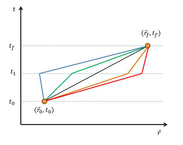
The interpretation of this equation is that $$K^+(1,0)$$ propagates from time $$t_0$$ to $$t_1$$ and, likewise, $$K^+(2,1)$$ propagates from $$t_1$$ to $$t_2$$. The one interesting feature is the sum over all possible positions $$\vec r_1$$ at the intermediate time $$t_1$$. A schematic representation of this equation is shown in this figure.
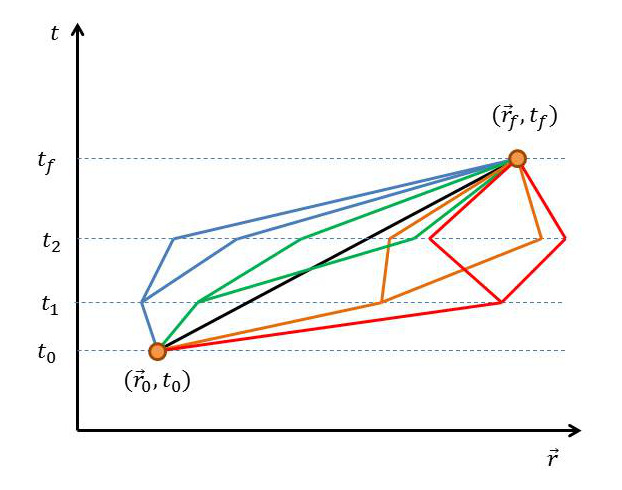
In an obvious fashion, the inclusion of a new time slice can be naturally accommodated with the corresponding propagation equation
\[ K^+(f,0) = \int d^3 r_1 \int d^3 r_2 K^+(f,2) K^+(2,1) K^+(1,0) \; .\]
and accompanying figure.
It is easy to extend this idea to infinite number of time slices and, in doing so, construct the Feynman path integral.
\[ K^+(f,0) = \lim_{N \rightarrow \infty} \int d^3 r_1 \int d^3 r_2 \int d^3 r_3 … \\ \int d^3 r_N K^+(f,N)… \; K^+(3,2) K^+(2,1) K^+(1,0) \]
As it stands, this form of the path integral doesn’t lend itself easily to computations. What is needed is a physical interpretation for the primitive term
\[ K^+(i,j) = \left< \vec r_i \right| U(t_i,t_j) \left| \vec r_j \right> \theta(t_i – t_j) \]
that affords a connection with physical models of motion that are easy to specify.
Sakurai states that this term, which he writes as
\[K^+(i,j) = \left< \vec r_i, t_i \right. \left| \vec r_j, t_j \right> \]
(with the implicit understanding that $$t_i > t_j$$) is the transition probability amplitude that a particle localized at $$\vec r_j$$ at time $$t_j$$ can be found at $$\vec r_i$$ at time $$t_i$$. He further describes the ket $$\left| \vec r_i, t_i \right>$$ as an eigenket of the position operator in the Heisenberg picture. Switching from the Schrodinger to Heisenberg pictures provides the mathematical framework that adds rigor to the heuristic concepts shown in the figures above. It provides a connection between the mathematical composition property of the propagator with an intuitive physical picture where paths in spacetime can be used to understand quantum evolution.
Sakurai also provides another vital ingredient, although he doesn’t draw the explicit connection that is presented here. Suppose that the wave function is expressed, without loss of generality, in the following way
\[ \psi(\vec r,t) = \rho(\vec r,t) e^{i S(\vec r,t)/\hbar} \; . \]
Plugging this form in the Schrodinger equation yields
\[ -\frac{\hbar^2}{2m} \left( \nabla^2 \rho + \frac{2i}{\hbar} \nabla \rho \nabla S + \frac{i}{\hbar} \rho \nabla^2 S – \frac{1}{\hbar^2} \rho (\nabla S)^2 \right) + V \rho = i \hbar \dot \rho – \rho \dot S \; .\]
Dropping all terms proportional to $$\hbar$$ results in
\[ \frac{ (\nabla S)^2 }{2 m} + V + \frac{\partial S}{\partial t} = 0 \; ,\]
which is the Hamilton-Jacobi equation with the phase of the wave function $$S$$ as the action. So there is a clear connection between the quantum phase and the classical concept of a path.
This connection can be pushed further by assuming that the transition amplitude is related to the action via
\[ \left< \vec r_i, t_i \right. \left| \vec r_j, t_j \right> \sim N \exp \left( \frac{i S}{\hbar} \right) \; ,\]
where $$N$$ is a to-be-determined amplitude. Is there any sense that can be made out of this equation? The answer is yes. With an inspired manipulation, the Schrodinger wave equation can be recovered. While I am not aware of how to do this in the most general case involving an arbitrary action, there is a well-known method that uses the conventional action defined in terms of the basic Lagrangian given by
\[ L = \frac{1}{2} m v^2 – V(\vec r,t) \; .\]
The trick is to concentrate on the propagation of the wave function between a time $$t$$ and time $$t+\epsilon$$ where $$\epsilon$$ is a very small number. In this model (and with $$t=0$$ for convenience), the wave function propagation takes the form
\[ \psi(\vec r_{\epsilon},\epsilon) = \int_{-\infty}^{\infty} d^3r_0 K^+(\vec r_{\epsilon},\epsilon;\vec r_0,0) \psi(\vec r_0,0) \]
Over this small time interval, the classical trajectory must be very well approximated by a straight line from $$\vec r_0$$ to $$\vec r_\epsilon$$. The Lagrangian becomes
\[ L = \frac{1}{2} m \left( \frac{\vec r_{\epsilon} – \vec r_0}{\epsilon^2} \right)^2 + V\left( \frac{\vec r_\epsilon + \vec r_0}{2},0 \right) \]
with the corresponding action being
\[ S = \int_{0}^{\epsilon} L dt = \frac{1}{2}m \frac{(\vec r_{\epsilon} – \vec r_0)^2}{\epsilon} + V\left( \frac{\vec r_\epsilon + \vec r_0}{2},0 \right) \; .\]
Plugging this into the assumed form for the propagator gives the following expression
\[ \psi(\vec r_{\epsilon},\epsilon) = N \int_{-\infty}^{\infty} d^3r_0 \exp \left( \frac{im}{2\hbar \epsilon} (\vec r_{\epsilon} – \vec r_0)^2 \right) \\ \exp \left( \frac{i \epsilon}{\hbar} V\left( \frac{\vec r_\epsilon + \vec r_0}{2}, 0 \right) \right) \psi(\vec r_0,0) \]
The strategy for simplifying this integral is fairly straightforward, even if the steps are a bit tedious. The core concept is to evaluate the integral by using a stationary phase approximation where only paths closest to the classical path are evaluated. The technical condition for this approximation is
\[ \frac{im}{2 \hbar \epsilon} (\vec r_{\epsilon}-\vec r_{0})^2 \approx \pi \]
Defining the difference vector $$\vec \eta = \vec r_{\epsilon} – \vec r_{0}$$, this condition can be re-expressed to say
\[ |\vec \eta| \approx \left( \frac{\pi 2 \hbar \epsilon}{i m} \right)^{1/2} \].
The next step is to expand everything to first order in $$\epsilon$$ or, where it appears, second order in $$\eta \equiv |\vec \eta|$$ (due to the relation between $$\epsilon$$ and $$\eta$$).
\[ \psi(\vec r_{\epsilon},\epsilon) = N \int_{-\infty}^{\infty} d^3 \eta \exp\left( \frac{im\eta^2}{2\hbar\epsilon}\right) \\ \left[ \left(1 -\frac{i\epsilon}{\hbar} V(\vec r_\epsilon,0)\right)\psi(\vec r_\epsilon,0) + \vec \eta \cdot (\nabla \psi)(\vec r_\epsilon,0) + \frac{\eta_j \eta_j}{2} (\partial_i \partial_j \psi)(\vec r_\epsilon,0) \right] \; ,\]
where
\[ \partial_i \partial_j \equiv \frac{\partial}{\partial r_i} \frac{\partial}{\partial r_j} \; .\]
The last step is to simplify using the following three Gaussian integrals:
\[\int_{-\infty}^{\infty} e^{-ax^2} = \sqrt{\frac{\pi}{a}} \; ,\]
\[\int_{\infty}^{\infty} x e^{-a x^2} = 0 \; ,\]
and
\[\int_{\infty}^{\infty} x^2 e^{-a x^2} = \frac{1}{2a} \sqrt{\frac{\pi}{a}} \; .\]
Note that, in particular, the action of the second integral is to kill the term $$\vec \eta \cdot \nabla \psi$$ and to eliminate all terms in $$\eta_i \eta_j \partial_i \partial_j$$ where $$i \neq j$$. Also note that the wave function inside the integral is expanded about $$\vec r_\epsilon$$.
Performing these integrals and simplifying, we arrive at the standard Schrodinger equation in the position representation
\[ \psi(\vec r,\epsilon) – \psi(\vec r, 0) = \frac{-i\epsilon}{\hbar} \left[ \frac{-\hbar^2}{2m} \nabla^2 + V(\vec r,0) \right] \psi(\vec r,0) \]
provided that we take
\[N = \sqrt{ \frac{m}{2 \pi \hbar i \epsilon} } \; .\]
Emboldened by this success, the now-accepted interpretation is that the path integral is evaluated according to the following recipe
- Draw all paths in the $$\vec r-t$$ ‘plane’ connecting $$(\vec r_f,t_f)$$ and $$(\vec r_0,t_0)$$
- Find the action $$S[\vec r(t)]$$ along each path $$\vec r(t)$$
- $$K(\vec r_f,t_f;\vec r_0,t_0) = N \sum_{all paths} e^{i S[\vec r(t)] / \hbar}$$
Next week, I’ll put that recipe into action for the free particle propagator.