Last month’s column introduced the notion of the thermodynamic square as a mnemonic for organizing certain second-order partial derivatives amongst the various thermodynamic potentials: the internal energy $$U$$, the Gibbs and Helmholtz free energies $$G$$ and $$F$$, and the enthalpy $$H$$. As previously alluded to, physicist primarily use these relations (called the Maxwell Relations) to eliminate the terms difficult or impossible to measure experimentally in favor of parameters that are easily measured in the lab.
A practical example of the application of the Maxwell relations is the simplification of the ‘first’ and ‘second $$T dS$$ equations’ as listed in Exercise 7.3-1 on page 189 of Herbert B. Callen’s book Thermodynamics and an Introduction to Thermostatistics, 2nd edition. The relevant physical properties in these equations are (Sec. 3.9 of Callen):
the number of particles $$N$$,
the differential heat $$dQ = T dS$$,
the heat capacity at constant volume $$c_V = \frac{T}{N} \left( \frac{\partial S }{\partial T} \right)_V= \frac{1}{N} \left(\frac{\partial Q }{\partial T}\right)_{V}$$,
the heat capacity at constant pressure $$c_P = \frac{T}{N} \left( \frac{\partial S }{\partial T} \right)_P = \frac{1}{N}\left(\frac{\partial Q}{\partial T}\right)_{P}$$,
the coefficient of thermal expansion $$\alpha = \frac{1}{V} \left(\frac{\partial V}{\partial T}\right)_P $$, and
\[ T dS = N c_V dT + \frac{T \alpha}{\kappa_T} dV \; .\]
From the form of this equation, assume that the quantity in question is the entropy as a function of the temperature and volume $$S = S(T,V)$$. Taking the first differential gives
Multiplying each side by $$T$$ gets us to the final form of the first $$T dS$$ equation
\[ T dS = N c_V dT + \left(\frac{T \alpha}{\kappa_T} \right) dV \; .\]
Second $$TdS$$ Relation
The second relation is
\[ T dS = N c_P dT – T V \alpha dP \; . \]
From the form of this equation, assume that the quantity in question is the entropy as a function of the temperature and pressure $$S = S(T,P)$$. As in the first $$T dS$$ relation, taking the first differential gives
Multiplying the second term by $$V/V$$ and simplifying gives
\[ dS = \frac{N c_P}{T} dT – V \alpha dP \; ,\]
which becomes the desired relation when multiplying both sides by $$T$$
\[ T dS = N c_P dT – T V \alpha dP \; .\]
To summarize, these two relations show how to express the heat $$T dS$$, expressed in terms of the entropy (which cannot be measured) in terms of parameters, such as temperature, pressure, and heat capacity, that are easily measured in the lab. All that is needed is the machinery of partial derivatives. This observation is the reason that so many textbooks on Thermodynamics have specific sections devoted to these approaches.
Last month’s installment presented a clean derivation of the classic relations between partial derivatives and showed a simple example of how they work in the concrete. As nice as that presentation is, the real power of these relations is only realized when dealing with systems with a large number of variables in play and in which various manipulations are required to extract meaning from the systems involved. The prototypical example is classical thermodynamics.
The fundamental concept in thermodynamics is the existence of a thermodynamic potential, which is a scalar function that encodes the state of the thermodynamic system in terms of the measurable quantities that describe the system, such as volume or temperature. Changes in the values, these independent physical variables (sometimes called the natural variables), relate directly to the potential of the corresponding partial derivatives.
The textbook example of this type of relation is defined in the first law of thermodynamics, which asserts that there exists a function, called the internal energy $$U$$, that is a function of the entropy $$S$$, the volume $$V$$, and the number of particles $$N$$ making up the physical system being modeled (assuming a single type of substance; generalizations to multiple species is straightforward but cumbersome). Changes in the internal energy $$U$$ can be calculated by
\[ dU = T dS – P dV + \mu dN \; ,\]
where the temperature, pressure and chemical potential are defined as
Without dwelling on the theory, suffice it to stay that laboratory conditions vary and there are many circumstances where it is preferable to work with a different set of independent variables. For example, heating water on a stove top in an uncovered pan is better understood in terms of fixed pressure rather than fixed volume.
Thermodynamics supplies an approach for dealing with these cases using the Legendre transformation. In the stove-top experiment mentioned above, the appropriate potential is called the enthalpy, defined as
\[ H = U + PV \; . \]
Taking the first differential gives
\[ dH = dU + P dV + V dP \\ = T dS – P dV + \mu dN + P dV + V dP \\ = T dS + V dP + \mu dN \; , \]
which demonstrates that $$H = H(S,V,N)$$.
Assuming that the order of differentiation can be exchanged, there are several relationships that exist (called Maxwell relations) between various partial derivatives. For example:
Obviously, there is a lot of notational overhead in the above relation. For the sake of this analysis, we will make two simplifications to improve the clarity. First, we will assume a single species with a fixed number of moles. This assumption removes the need to carry $$N$$ and $$\mu$$. Second, we will forego keeping track of the other variables being held constant. Since we will be tacitly tracking which thermodynamic potential is being used, there is little chance of confusion.
The primary purpose the Maxwell relations serve is to eliminate terms involving the entropy in favor of physical parameters that can be experimentally measured, such as temperature, volume, or pressure.
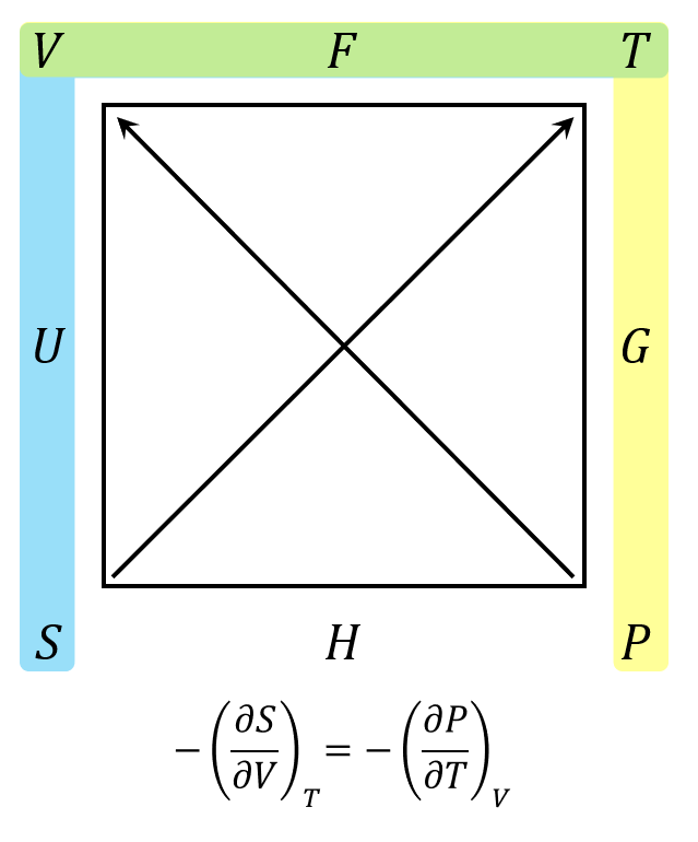
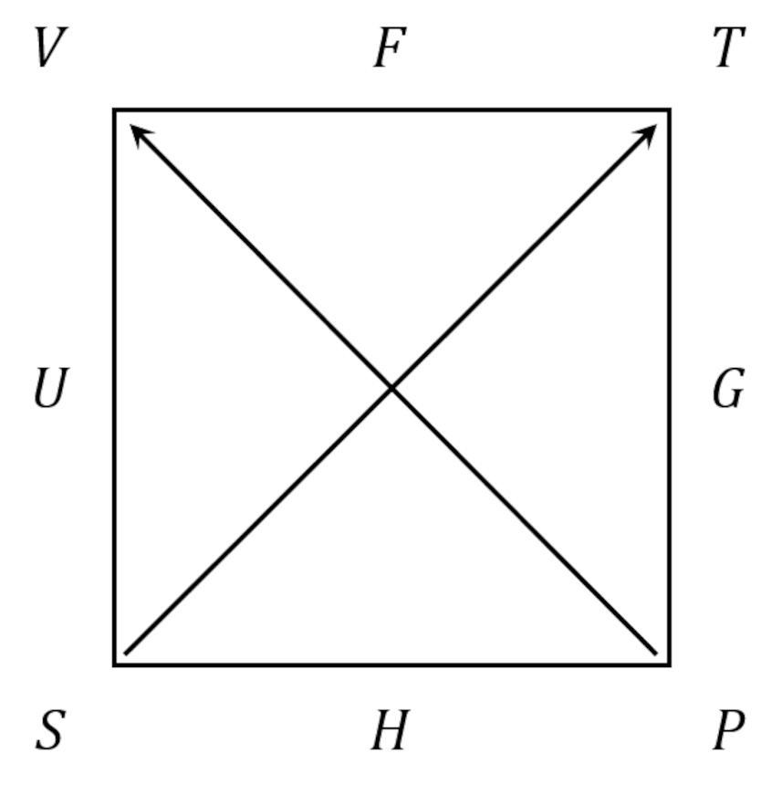
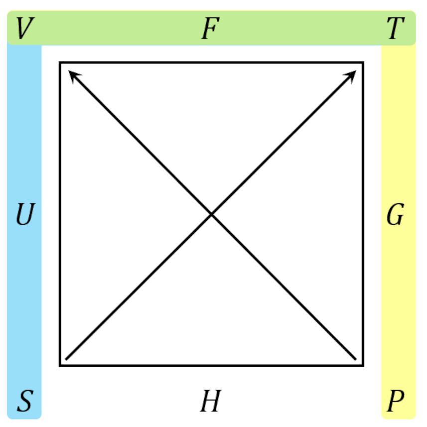
A useful mnemonic exists for looking up the various relations without scanning through a table. It’s called the thermodynamic square, and it’s constructed as below
The 4 most important thermodynamic potentials, the Helmholtz free energy $$F = U – TS$$, the Gibbs free energy $$G = U + PV – TS$$, the enthalpy $$H = U + PV$$, and the internal energy $$U$$, are arranged along the edges starting up at the top and going clockwise. The thermodynamic variables – the temperature $$T$$, the pressure $$P$$, the entropy $$S$$, and the volume $$V$$ – are arranged at the corners, starting just after $$F$$ and also going clockwise. The Maxwell relations relate a partial derivative expressed in terms of three consecutive corners (shaded blue below) to the partial derivative expressed in terms another three consecutive corners (shaded yellow). The arrows lying along the diagonal set the sign of the partial derivative based on which variable is in the numerator: those with the arrowhead positive and those without negative.
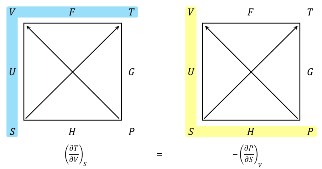
These rules are far easier to understand with the mixed partial derivatives of $$U$$ discussed above.
The blue shaded region reads counterclockwise while the yellow region reads clockwise. These orientations follow from the overlap they share on the left-hand side of the square (the one labeled $$U$$). The signs are determined by the arrows. Since the $$T$$ corner is the numerator and it has an arrowhead, the partial derivative is positive. Likewise, since the $$P$$ corner is the numerator and it lacks an arrowhead, the partial derivative is negative.
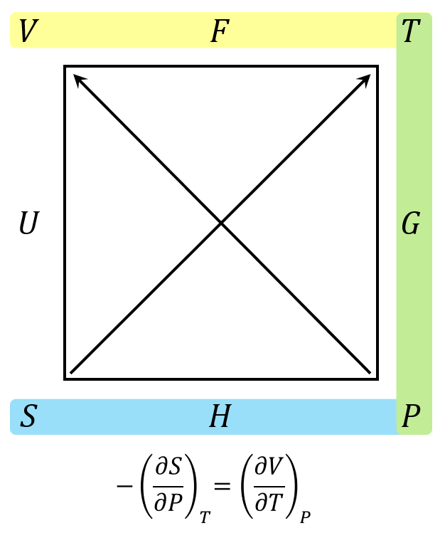
Once the basic operations using the square are understood, it is easier to present a single square with the common side being both shaded in blue and yellow, resulting in green. An example for the Maxwell relations coming from the Helmholtz free energy $$F$$ being
With these tools, we can get to the meatier topics, namely using a combination of the classical rules for partial derivatives and the Maxwell relations, as presented in the thermodynamic square, to eliminate the entropy in favor of physically measurable quantities. But this will be the topic for next month’s post.
Partial derivatives are an important mathematical tool in a number of physics disciplines, most notably field theories (e.g. electricity & magnetism and general relativity) and in thermodynamics.
However, working with partial derivatives are always a bit tricky and teaching students about them is usually fraught with difficulties. So it was to my pleasant surprise that I found a really nice discussion of how to derive the various ‘classic’ rules cleanly presented in Classical and Statistical Thermodynamics by Ashley H. Carter.
My presentation here is strongly influenced and closely follows her presentation in Appendix A, although I’ve added on a bit in the theoretical flow and I’ve also provided explicit examples in terms of the standard paraboloid found in freshman calculus.
Assume a function of 3 variables can be expressed as $$f(x,y,z) = 0$$. This equation can be viewed as a constrain equation linking the values of the variables such that two variables are independent. That means that we can (at least locally) solve for:
$$x(y,z) = 0$$
$$y(x,z) = 0$$
$$z(x,y) = 0$$
Focus on the first and second forms (other pairings will follow a simple relabeling of the variables). The corresponding differentials are
Let’s take a look at these relationships in action. Consider the implicit definition of the paraboloid
\[ x^2 + y^2 – z = 0 \; . \]
As mentioned earlier, this equation can be considered as a constraint equation that selects out a value for any one of the three variables given the other two. In other words, we can imagine a look up table where we select a value of $$x$$ and $$y$$, we rummage through the table to find a row with both values and then we scan to the right to find the allowed value of $$z$$ that makes it satisfy the implicit equation.
How do you construct this table; not at a finite set of points but functionally so that it works at any point? It is natural and easy to determine $$z$$ given $$x$$ and $$y$$ by simply rewriting the implicit equation as
\[ z(x,y) = x^2 + y^2 \; .\]
However, it isn’t as easy to express $$x$$ or $$y$$ as functions of the remaining two variables because of the two possible signs that result from taking the square root. We need to have four functional relationships
depending on the particular combination of whether $$x$$ is positive or negative and whether $$y$$ is also positive or negative. In the language of differential geometry, we have a 5 charts in our atlas.
We are now in position to try the various relations derived above. For example, let’s examine the reciprocal relation in the first quadrant of the $$x$$-$$y$$ plane. We need to use $$x_p$$ as our local chart.
where there is no need for the $$z$$-chart to distinguish between positive and negative values of $$x$$. As expected the derivatives are reciprocals of each other.
Next, let’s test the fraction rule. For fun, this time let’s test it in the 2nd quadrant in the $$x$$-$$y$$ plane ($$x < 0$$ and $$y > 0$$). Calculating the partial derivatives on the left-hand side yields
Finally, for the cyclic rule, let’s go into the 4th quadrant in the $$x$$-$$y$$ plane ($$x>0$$ and $$y<0$$). Taking each partial derivative in turns yields
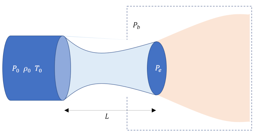
In this final post on compressible fluid flow, we will take a look at an application of the machinery developed over the previous three posts to the converging-diverging nozzle, often called a rocket nozzle or a de Laval nozzle. The setup in straightforward even though it is probably unfamiliar. We imagine a reservoir containing a gas at a high pressure and, not often, high temperature that serves to supply the flow through the nozzle. By convention, the thermodynamic state variables in the reservoir are given a ‘0’ subscript and are called the stagnant conditions as there is no flow within the reservoir itself. This reservoir feeds into a converging section of a nozzle in which the cross-sectional area decreases steadily until a minimum occurs at what is called the throat of the nozzle. After the throat, the cross-sectional area increases again until the nozzle ends at the exit. The nozzle and reservoir are placed into a larger pressure vessel (sometimes called the receiver) where the pressure outside of the exit, called by convention the back pressure, $P_b$.
Initially the two pressures are equal and there is no flow from the reservoir through the nozzle. As the back pressure is dropped, flow develops from the reservoir. de Laval’s innovation was to realize that if the flow can be brought to sonic conditions (i.e., Mach number $M=1$) at the throat then the diverging section would further speed up the flow to supersonic speeds (see the discussion at the end of the second post of this series).
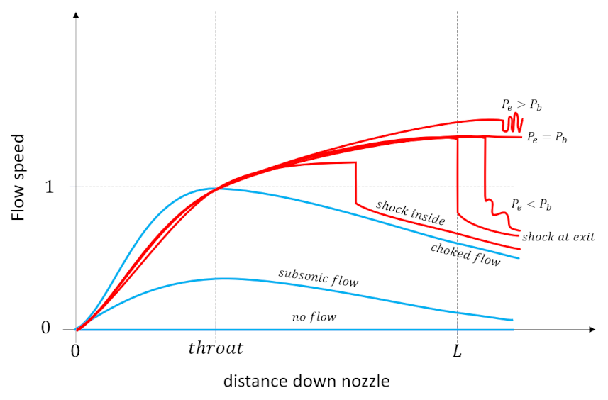
The goal of this post is to discuss the flow profiles along the length of the nozzle, from inlet at the reservoir, to exit into the pressure vessel, as a function of the ratio $P_b/P_0$ and to give a flavor of how the previous equations are used to quantitatively. Despite the relative simplicity of the system (reservoir, nozzle, and pressure vessel) a rich set of flow patterns result. Qualitatively, these fall into two broad classes with several variations within them.
In the first class (shown in blue traces in the figure below), the flow is everywhere isentropic from the reservoir. through the nozzle, and into the pressure vessel. Included in this class is the flat trace where $P_b/P_0 = 1$ where no flow results. As $P_b/P_0$ is lowered, flow commences with the speed of the flow increasing as it approaches the throat from the converging section and then subsequently slowing down in the diverging section. The maximum speed in the nozzle (which for this class is always at the throat) continues to increase until as $P_b/P_0$ is lowered until a critical value of the back pressure, $P_{b_s}$ when the flow is sonic (i.e., $M=1$) in the throat but still subsonic everywhere else in the nozzle (including the diverging section).
At this point, lowering the $P_b/P_0$ ratio further develops the second class of flow (shown in red traces in the figure below) where some portion of the flow in the diverging section is supersonic. A shock develops somewhere downstream of the throat in order to decelerate the flow back to subsonic conditions so that it can match boundary conditions with the environment in the pressure vessel. The only remaining question is precisely where the shock is found. Five possible options are available: 1) the shock is found in the nozzle between the throat and the exit, 2) the shock falls at the exit, 3) the shock is beyond the nozzle but the exit pressure $P_e < P_b$, 4) the shock is beyond the nozzle and $P_e = P_b$, and 5) the shock is beyond the nozzle but $P_e > P_b$. Options 3), 4), and 5) are called over-expanded, perfectly-expanded, and under-expanded flows, respectively (see discussion of The Converging-Diverging Nozzle applet).
In the third post of this series, we derived expressions relating the pressure, density, and temperature anywhere in an isentropic portion of the flow to the stagnation properties in the reservoir. The relations derived were:
that specified what the ratio of the local area, $A$, to the area of the throat, $A^*$, must be to achieve a target value of Mach number $M$. A typical problem where these equations are useful comes from Fluid Mechanics Demystified by Merle Potter and reads
Air flows through a converging-diverging nozzle attached to a reservoir maintained at 400 kPa absolute and 20$^{\circ}$C to a receiver. If the throat and exit diameters are 10 and 24 cm, respectively, what is the receiver pressure that will just result in supersonic flow throughout the diverging portion of the nozzle.
The solution starts with recognizing that if the flow in the diverging portion of the nozzle is to be supersonic then choked conditions occurs at the throat and, as a result, the throat area coincides with the critical area $A_{throat} = A^*$. The area ratio of the exit to the throat is then $\frac{A}{A^*} = \left( \frac{24}{10} \right)^2=5.76$. Next we have to invert the AMR to find the value of $M$ that corresponds to this ratio. A bisection, specifically adapted to the two possible dynamical behaviors: subsonic and supersonic, was written in python. The resulting value was $M=3.3244$ was then plugged into the $P_0/P$ relation and the reciprocal taken to arrive at the exit pressure being $P_{exit} = 6746.659 \, Pa$, corresponding to an exit pressure only about $1.6%$ as large as the stagnant pressure.
The possibility of a shock in the possible flows requires us to add three new relations to our collection. Our starting point for deriving the so-called jump conditions across the shock are the three basic fluid equations for mass, momentum, and energy, derived in the first post, but simplified by the tacit assumption that the shock is negligibly thick so that the cross-sectional area is the same on both sides of the shock, giving:
respectively. Note that the subscripts `u’ and `d’ stand for upstream and downstream, respectively.
As before, our thermodynamics will assume the fluid to be an ideal gas with the equation of state given by $P/\rho = R T$. The general form of enthalpy $h = e + P/\rho$ takes the simple form $h = (\gamma/\gamma-1) P/\rho$. The state variables relate to their values at different parts of the flow via
The speed of sound in the gas, which is temperature dependent, takes on the forms
\[ c = \sqrt{\gamma R T } = \sqrt{\frac{\gamma P}{\rho}} = \sqrt{(\gamma-1) h} \; , \]
each useful in context.
Finally, the energy equation, which had been relegated to a by-stander role in incompressible fluid flow, offers two very useful relations. The first, which will be termed the stagnant enthalpy expression (SEE), expresses the stagnant enthalpy in terms of the local sound speed via $(\gamma -1) h = c^2$ giving
One caution when using these relations. The reservoir is operational defined as the location where the flow is isentropically brought to a stop. Since a shock produces a great deal of entropy for any fluid element crossing from one side to another, the downstream thermodynamic conditions for a reservoir will be different from the actual reservoir attached to the nozzle and care must be taken not to confuse the notional one with the actual physical one.
To derive the normal shock relations, we follow these notes.
Begin by dividing the momentum equation by the mass continuity equation to get
Next, employ a neat trick by writing the numerator on the left-hand side as ${h_0}^2 (\gamma-1)^2 = h_{0u} (\gamma-1) h_{0d} (\gamma – 1) $. Use the SEE to express each of these expressions in terms of the local sound speed and Mach number. Doing so yields
Solving for $M_d$ is relatively painless with the substitutions $L = (\gamma-1)/2$ and $Q = (\gamma +1)/2$. These auxiliary variables keep the clutter down and the observation that $L^2 – Q^2 = -\gamma$ simplifies things enormously so that we arrive at
Earlier in the derivation of the Mach jump relations we found that $1/V_u V_d = (\gamma+1)/2 h_0(\gamma-1)$. Substituting these expressions back into the density equation yields
Using the already obtained expression for the density ratio (and noting to flip it based on which density is in the numerator) followed with some simplifications gives
We are now in a position to solve another typical problem associated with converging-diverging nozzle design, again taken from Merle Potter, that reads
Air flows from a reservoir through a nozzle into a receiver. The reservoir is maintained at $400 kPa$ absolute and $20{}^\circ C$. The nozzle has a 10-cm-diameter throat and a 20-cm-diameter exit. What is the back pressure that locates the shock wave at the exit?
Since the shock is at the exit, we can assume that the upstream side of the shock is supersonic at the area of the exit. So, the value of $A/A* = 4$. Using the inverse AMR function, the upstream Mach number is $M_u = 2.940$. Then using the standard isentropic relations the pressure ratio is $P_u/P_0 = 0.0298$ resulting in an upstream pressure of $P_u = 11,914.79 Pa$. Finally, the Mach shock jump relationship yields $P_d/P_u = 9.919$ for a downstream pressure, which is equal to the receiver pressure, of $P_d = 118179.93 Pa$.
Of course, this analysis just barely scratches the surface but these basic relations demonstrate the interplay between three basic laws of fluid mechanics: continuity, momentum, and energy and how they contribute to the practical construction of a converging-diverging nozzle. And, so, I guess this is rocket science.
This month’s column, the second in a series of three on compressible flow, derives the key relationships for understanding steady, isentropic flow in a converging-diverging nozzle. The starting point of these derivations are the three isentropic jump conditions derived in the last post:
along with the first law of thermodynamics (cast in intensive variables by dividing both sides of $dE = TdS – P dV$ by mass $m = \rho V$)
\[ de = T ds + \frac{P}{\rho^2} d \rho \; ,\]
and the equation of state for an ideal gas (also in intensive variables)
\[ \frac{P}{\rho} = R T \; . \]
The $T ds$ term can be dropped since isentropic flow means that the specific entropy remains constant. Note that the specific internal energy and specific enthalpy ($h = e + P/\rho$) are simply functions of temperature given by $de = c_{{\mathcal V}} dT$ and $dh = c_P dT$, respectively, where $c_{{\mathcal V}}$ and $c_P$ are the heat capacities at constant volume and constant pressure and are taken to be constants. Other thermodynamic relations will be taken as given since proof will take us too far afield.
There are three ingredients in understanding the steady, isentropic flow through a converging-diverging nozzle (also known as a de Laval nozzle): 1) calculating the Mach number, 2) relating the cross-sectional area of the nozzle ($A$) to the Mach number, and 3) relating the thermodynamics variables of temperature ($T$), the pressure ($P$) and the density ($\rho$) to the Mach number. This post will deal with items 1 and 2 with item 3 being covered in the next post.
This post and the next are a synthesis and clarification of the ideas and materials found in Chapter 9 of Merle Potter’s Fluid Mechanics Demystified and the 5-part series of YouTube lectures on compressible fluid flow from the University of Florida (part 1, part 2, part 3, part 4, and part 5)
Calculating the Mach Number
The central parameter in the theory is the Mach number, which is innocently defined as the ratio of the flow speed to the speed of sound. What makes this definition so deceptively simple looking is we are used to thinking that the speed of sound is constant since the temperature range that we normally encounter is such that the variations in the speed of sound is negligible. However, interesting compressible fluid flows often have very large variations in temperature over short durations or small distances and so Mach number varies depending on the location of the flow within the nozzle.
To calculate the speed of sound, which we will denote as $c$, we take the first differential of the continuity and momentum equations and since we are interested in the local speed over a column of fluid with constant cross section we can ignore variations in the area (imagine being outside). The resulting equations are:
\[ d \rho c + \rho d c = 0 \; \]
and
\[ d\rho c^2 + 2 c \rho dc + dP = 0 \; . \]
Solving the first equation for $\rho dc = – c d \rho$, substituting this result into the second, and solving for $c^2$ gives
Substituting this result back into the first equation and taking the square root gives
\[ c = \sqrt{ \frac{\gamma P }{\rho} } = \sqrt{\gamma R T} \; , \]
where the ideal gas law was used in the last step.
The Mach number is the ratio of the flow speed to the speed of sound and is given by
\[ M = \frac{V}{c} \; . \]
Relating Cross-Sectional Area and the Mach Number
Most of us have had the experience with running water where we restrict the cross-sectional area of the outlet and watch the fluid flow increase (a thumb over the end of a garden hose being the usual scenario). The reason for this speed increase is that the pressure difference between the inlet and the outlet sets up a given mass flow rate. When the area drops, the flow speed has to increase to maintain that flow rate.
This approach works for flows in most everyday experiences but fails for compressible flow, explaining why a simple converging nozzle is insufficient to force a fluid into supersonic flow.
To see why this is we will derive a relationship between the cross-sectional area and the Mach number.
Start by taking the first differential of the third jump condition
\[ d \left( h + \frac{V^2}{2} \right) = dh + V dV = 0 \; .\]
Next, eliminate the differential of the enthalpy using the first law ($dh = dP/\rho$) to get
\[ \frac{dP}{\rho} + V dV = 0 \; .\]
Multiply the first term by $d\rho/d\rho$ to get
\[ \frac{dP d\rho}{\rho d\rho} + VdV = 0 \; .\]
Recognizing that $c^2 = dP/d\rho$ and dividing both sides by $V^2$ gives
When $M > 1$ the flow slows down (speeds up) when the area decreases (increases) When $M < 1$ the flow speeds up (slows down) when the area decreases (increases) When $M = 1$ the flow remains at the same speed even as the area changes
These observations explain why a simple converging nozzle can’t force the flow to supersonic speeds. Once the pressure difference between the inlet and outlet is large enough that the flow speed equals the speed of sound ($M=1$), the flow is choked and can get no faster. Practitioners usually speak of this situation is that choked flow can’t communicate a further pressure drop at the outlet upstream so that the flow can respond.
It is also worth pointing out something that is easy to overlook in the above manipulation. While the steps may seem haphazard and uninspired there is a method to the madness. There is a hierarchy of thermodynamic relations that are combined: the first law of thermodynamics is a universal law; the third jump condition represents energy conservation for a general fluid flow; and the equation of state for an ideal gas is a specific law for a very special kind of fluid. The first law links a fluid’s energy conservation with the speed of sound for an ideal fluid, linking flow velocity to Mach number and the compressibility of the fluid (as represented by $d\rho$). The final step uses another universal law – mass continuity – to arrive at a relationship between a fractional change in the flow speed to a fractional change in volume (as represented by $dA$).
Next post puts these pieces together with a set of relations between the fluid’s thermodynamic variables and the Mach number to explain the function of a converging-diverging nozzle and how it can push fluid flows past the speed of sound.
This month’s column briefly examines compressible fluid flow. This journey will be a short excursion into a rather complicated discipline with only two aims. The first is to give a flavor of how and why the energy equation, which has been essentially unused in previous analyses, plays a role and how additional thermodynamic information (spatial and temporal variations in density and temperature) comes into play. The second is to setup all the equations needed to understand the basic physics associated with that object that ushered in the space age: the rocket nozzle, which will be the subject of next month’s entry.
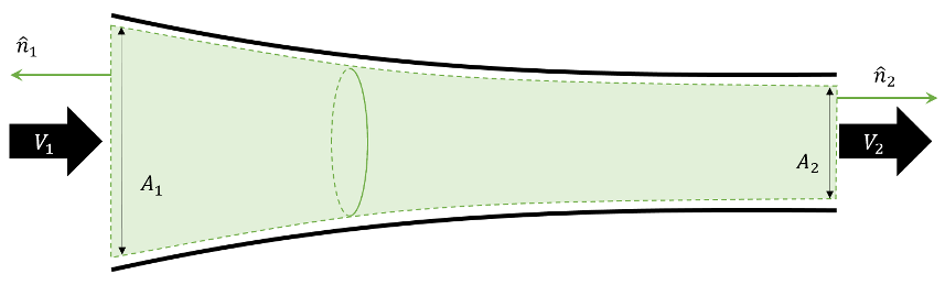
Following the usual introductory approaches (e.g. Eric R. Pardyjak’s online notes and Chapter 9 of Merle C. Potter’s Fluid Mechanics Demystified), we will look at only simplified geometries, such as the converging nozzle shown here
with a flow from left-to-right as indicated.
This analysis assumes that all of the flow variables are constant over each cross-section but can differ from cross-section to cross-section. The first condition means that the flow is effectively inviscid, since the boundary layer is ignorable for the vast majority of the flow, and it is steady. All of these simplifying assumptions result in algebraic flow equations that come from the integral forms of the fluid equations rather than the differential equations. In addition, we will ignore body forces (i.e. gravity) and only allow pressure-driven flows.
The conservation (i.e. Eulerian) form of the equations is slightly easier to work with and these will be our starting point for the various simplifications that we impose (although with one extra wrinkle in the case of energy). All of the derivations will involve some vector quantity (say the velocity $${\vec V}$$) being integrated over a surface after being projected onto the local surface normal. This process results in an average value of the normal component of the vector over the entire face. This quantity will be denoted simply as a scalar (e.g. $$V_1$$) with appropriate labeling indicating which segment of the bounding surface.
Since the flow is steady, the first term vanishes. If we imagine the surface as shown in the nozzle above, then only the flow through the endcaps ($${\mathcal S}_1$$ and $${\mathcal S}_2$$) is non-zero and
where $${\mathbf T}$$ is the Cauchy stress tensor. Following the same approach as above, and recalling that the body forces are zero (i.e. $${\mathbf T} = – P {\mathbf I}$$), the Cauchy momentum equation takes the form:
where we’ve used $${\hat n}_1 = – {\hat n}_2$$. Two things are worth noting about this equation. First, the direction of the flow must be along (either parallel or anti-parallel) to the end-caps, nicely in keeping with the assumption that the flow varies only from cross-section to cross-section and not within a cross-section. Second, the continuity equation can be used to eliminate many of the terms in favor of the constant mass flow rate $${\dot m}$$. Keeping all this in mind brings us to the scalar equation
Up to this point, we’ve not had to occasion to use the energy equation for the simple fact that in incompressible flows without explicit heat flows and generation, the internal energy of each fluid element remains constant; only the kinetic energy changed. Indeed, the energy equation for such a flow follows immediately by taking the dot product of the Cauchy momentum equation with the velocity. In these simple cases, the density is a given and only pressure and velocity are unknown. The four equations of continuity and 3 components of the Cauchy momentum equation sufficed to solve for the four unknowns.
Once we allow the flow to be compressible, the density becomes an unknown and the also the internal energy enters into the picture. The energy equation provides one more equation. The final equation comes from a thermodynamic equation of state. For this latter equation, we will assume the ideal gas law. Often, it is more convenient to switch from internal energy to temperature by using the ideal gas relation
\[ e = c_v T \]
and
Fourier’s law relating heat flow to temperature via
\[ {\vec q} = – k \nabla T \; .\]
There is an additional thermodynamic consideration (the one wrinkle mentioned at the beginning of this post). It is the introduction of the enthalpy $$h = e + P/\rho$$ that combines the internal energy with the pressure work. Its introduction is really a matter of convenience rather than an important insight but, as the majority of the discipline’s practioners uses it, it would be a mistake to omit.
To see how the energy equation admits its inclusion, start with the energy equation in its full glory
By the above assumptions, the volumetric heating and the heat flow are zero, the body forces are zero, the stress tensor simply accounts for the pressure, and the flow is steady. Under these conditions, the equation reduces to
This month’s column finishes up the study of elementary viscous flow and presents the final two examples, both dealing with shear-induced flow. This type of flow (called Couette flow) typically results from the no-slip condition in which a moving boundary drags the fluid that touches it into motion. That layer of the fluid then drags the fluid layer next to it and so on.
For both of these examples, we are going to ignore body forces and external pressure differences and focus on the boundary motion alone. These assumptions eliminate several terms from the incompressible Navier-Stokes equations leaving us with
augmented with the usual incompressibility assumption $$\nabla \cdot {\vec V} = 0 $$.
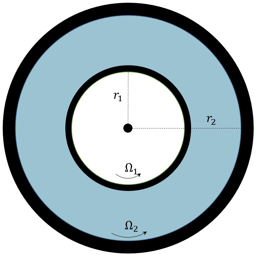
Cylindrical Couette Flow
In this example, we imagine a fluid trapped between two cylindrical shells, an inner and an outer shell, of radii $$R_{inner} \equiv R_{1}$$ and $$R_{outer} \equiv R_{2}$$, respectively.
For sake of generality, both shells will be allowed to rotate about the vertical axis (out of the page) with angular velocities $$\Omega_{inner} \equiv \Omega_{1}$$ and $$\Omega_{outer} \equiv \Omega_{2}$$. We seek to describe the velocity profile of the fluid in steady motion. With the radii and angular velocities assumed to be known there will be a fairly simple relationship between the velocity profile and the kinematic viscosity $$\nu$$. A viscometer uses this experimental setup to measure kinematic viscosity by tracking the torque required to keep the inner shell moving at a constant rate (the out shell is usually fixed).
The Navier-Stokes equations are best presented in cylindrical coordinates since these coordinates match the geometry involved. The added benefit is that expressing the derivatives in cylindrical coordinates is instructive in its own right.
The key point to focus on is that in cylindrical coordinates, the basis vectors in directions perpendicular to the $$z$$-axis change as a function of azimuthal angle $$\theta$$. The radial unit vector changes as
Note that the incompressibility condition is automatically satisfied by the form of the velocity field.
From the last equation the pressure cannot be a function of $$z$$ and since everything else in the second equation is only a function of $$r$$ so must $$\partial_{\theta} P = f(r)$$. Integrating gives
\[ P(r) = f(r) \theta + g(r) \; , \]
the form of which requires $$f(r) = 0$$ otherwise the pressure would be a multi-valued function. The second equation now becomes
which are easily obtained by applying the boundary conditions to the general relation $$V_{\theta} = r \Omega$$.
Once $$V_{\theta}$$ is known, the first equation gives the radial pressure gradient due to the rotation.
Linear Couette Flow
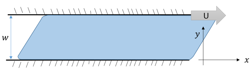
In this last example, we will solve the time varying Couette flow setup up between two plates separated by a distance $$w$$ and extending far in the $$x$$- and $$z$$-directions so that we can ignore the edge effects and model the flow as two-dimensional.
We imagine that the fluid is at rest prior to $$t=0$$ at which time the upper plate is set into motion with velocity $${\vec V} = U {\hat e}_x$$. There is a well-known steady solution in which the velocity linearly varies from zero on the lower plate to $$U$$ on the upper plate but it is interesting to see how the transient flow settles into this steady state.
By our earlier, assumptions, the flow is of the form (automatically satisfying the incompressibility condition)
\[ {\vec V} = V_x(t,y) {\hat e}_x \; , \]
which has to satisfy the following form of the Navier-Stokes equations
\[ \textrm{IC:} \;\;\;\;\;\;\;\; V_x(0,y) = 0 \;\;\;\;\; 0 \leq y \leq w \; , \]
respectively.
The solution strategy is to employ separation of variables. To that end, following Acheson, write the velocity as a sum of the steady solution and a time-varying piece where the latter has homogeneous boundary conditions
\[ V_x(t,y) = \frac{U}{w} y + {\tilde V}_x(t,y) = \frac{U}{w} y + f(t)g(y) \; . \]
After performing the separation of variables, we arrive at
\[ \frac{1}{\nu} \frac{1}{f} \partial_{t} f = – s_{n}^2 = \frac{1}{g} \partial_{y}^2 g \; , \]
where $$s_n$$ is a separation constant.
The spatial equation, $$g^{\prime\prime} + s_{n}^2 g = 0$$ has general solutions $$g(y) = A \sin (s_n y) + B \cos (s_n y) $$. Applying the boundary conditions requires $$B=0$$ and $$s_n = n \pi / w \;\; n = 1, 2, 3, \ldots$$. The time equation is easily integrated to $$f(t) = \exp( -s_n\nu t )$$. The general solution is
\[ V_x(t,y) = \frac{U}{w} y + \sum_{n=1}^{\infty} A_n \exp \left( – \frac{ n^2 \pi^2}{w^2} \nu t \right) \sin \left( \frac{n \pi}{w} y \right) \; . \]
The initial conditions are satisfied by picking the $$A_n$$ appropriately. The key to doing this is to exploit the orthogonality
\[ \int_0^w \sin \left( \frac{m \pi}{w} y \right) \sin \left( \frac{n \pi}{w} y \right) = \frac{w}{2} \delta_{mn} \; \]
to get
\[ A_m = -\frac{2}{w} \int_0^w \frac{Uy}{w} \sin \left( \frac{m \pi}{w} y \right) dy = \frac{ 2 U (-1)^n }{n \pi} \; . \]
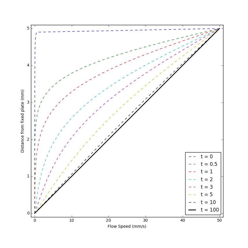
The following plot shows this solution for $$w = 5mm$$ and $$\nu = 0.8926 mm^2/s$$.
Note the majority of the velocity is confined near the top plate at short times (this is essentially the boundary layer) but how quickly the solution tends to the steady state.
As a way of seeing this boundary layer as a feature of the transient behavior consider what happens if the top plate moves in an oscillatory fashion with velocity $$U \cos (\omega t) $$. Assuming that the fluid velocity has the form $$ V_x(t,y) = f(y) e^{i \omega t} $$, the Navier-Stokes equations yield
\[ f” – i \omega/\nu f = 0 \; .\]
Following the usual strategy $$f = exp(\lambda y)$$ gives values
\[ V_x(t,y) = U e^{-ky} e^{i (\omega t – k y) } \; ,\]
where $$k = \sqrt{\omega/2 \nu}$$. As the following animation shows, the velocity at the upper plate follows the motion of the plate but the main action is confined to a thin layer. Essentially, the motion is always transient and the influence of the fluid motion near the moving plate isn’t able to diffuse into the bulk of the fluid.
This month’s column deals with viscous flow in a variety of situations. Three main physical effects can drive elementary fluid flow: the pull of gravity coaxing a fluid downhill; a pressure differential, such as in a pipe, causing the fluid to flow from inlet to outlet; or shearing motion, which, in the usual scenario, involves a moving boundary dragging the fluid. We’ll be looking at four examples covering different aspects of these three effects. The first two will illustrate the effect of gravitational body forces and pressure differentials to drive the fluid and will be covered in this column. The next two examples deal with steady and unsteady shear-induced flows and will be featured next month.
But, before we deal with specific examples, we will need to settle on a model of the fluid. Usually, when seeking analytic solutions describing the motion of non-ideal Newtonian fluids (already a simplification compared to the amazingly rich and diverse types of fluids that nature offers), one either chooses to assume the flow is viscous and incompressible or that it is inviscid and compressible. For these examples, we will choose the former.
The starting point will be the incompressible Navier-Stokes equations, of which the flux-conservative form is
Applying the incompressibility assumption ($$\nabla \cdot {\vec V} = 0$$) is easy to do using the Lagrangian form of the equations, but it is more instructive to play with the flux-conservative form. Most of the action takes place on the left-hand side so let’s focus on that by expanding the terms to get
where the first expression is the full continuity equation and the second is what is left after the incompressibility assumption is applied. The left-hand side is now simply
The third term on the right-hand side vanishes due to the incompressibility assumption. Dividing by the density gives the general form of the Navier-Stokes equations for incompressible fluid flow:
This equation is what we will use in the following examples.
Gravity-driven Flow
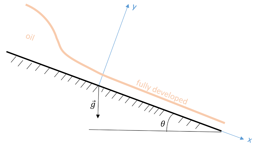
This example derives from the very nice YouTube lecture by Rick Sellens. Here we imagine flow of a fluid, such as oil, down an inclined plane (flow in the $$x$$ direction), as shown in the figure below. The height of the oil is larger at the top of the ramp but it quickly thins as gravity accelerates the oil. Eventually, the viscous force equals the component of the gravitational force parallel to the plane and, thereafter, the height of the oil is constant (the flow is said to be fully developed) and the velocity profile depends only on $$y$$. Once the flow establishes itself, this height profile remains constant in time and the flow is steady, allowing us to set all time derivatives to zero. We will assume that the incline is wide enough in the $$z$$-direction (not pictured) that we can approximate the flow as being two-dimensional. Next, we will confine our description to the fully developed portion of the flow ($$x > 0$$). Finally, we will assume a no-slip boundary condition at the incline plane and, since the flow is open to the air on top and air is not particularly viscous, we will assume the shear stress on the upper surface to be zero.
Applying the steady, fully-developed, and 2-D flow assumptions leads to the continuity equation
\[ \partial_x V_x = 0 \; \]
and the $$x$$- and $$y$$-component Navier-Stokes equations of
where $$g_x = g \sin(\theta) $$ and $$g_y = g \cos(\theta)$$, are the components of the gravitational acceleration parallel and perpendicular to the surface of the incline, respectively.
The continuity equation merely confirms what we already assumed, $$V_x = V_x(y)$$. The $$y$$ component of Navier-Stokes says that the pressure at the surface of the incline is higher than at the top due to the weight of the oil above. All the action is in the $$x$$-component equation.
The constant of integration is identically zero after the application of the no-slip boundary condition at the incline ($$V_x(y=0)=0$$).
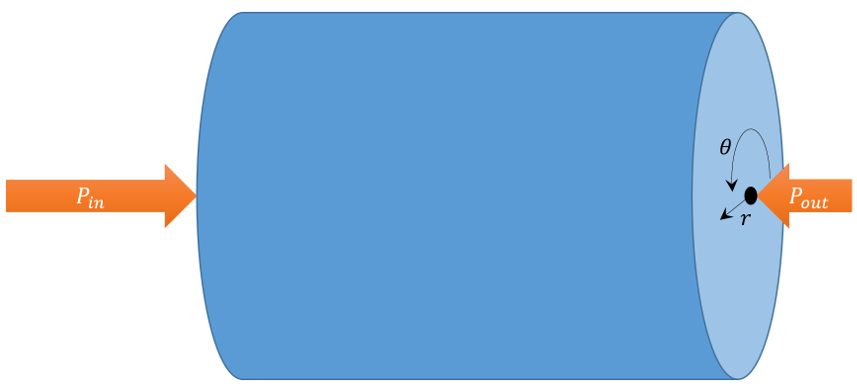
Pressure-driven Flow
This example draws from the Faculty of Kahn video on Poiseuille’s law. In this scenario, we imagine a horizontal pipe with an inlet pressure, $$P_{in}$$, and an outlet pressure, $$P_{out}$$, with $$P_{in} > P_{out}$$ and that the flow has had time to become steady. Cylindrical geometry clearly suggests itself and we expect that the only flow is in the $$z$$-direction ($$V_r = V_{\theta} = 0$$) and its only variation is radial ($$V_z = V_z(r)$$).
As discussed in an earlier post, usually one must take care to differentiate the basis vectors as well as the components when setting up fluid equations in curvilinear coordinates. However, the above assumptions are sufficiently limiting that only the $$z$$-component equation survives in the form
The constants of integration follow from a boundary condition that requires $$V_z(r=0)$$ to be finite and the usual no-slip boundary condition at the walls. The final form is then
Integrating this form over the surface area of the pipe gives the famous Poisueille flow rate relationship that says, for a given flow rate, the pressure differential is inversely proportional to the radius to the fourth power. This relationship has profound consequences in the field of medicine.
This month’s column begins a new chapter in the ongoing study of fluid dynamics. Up to this point, the general equations of fluid motion have been derived from Newton’s laws using the transformation between a fluid-following viewpoint (Lagrangian point-of-view) and a field concept (Eulerian point-of-view). General considerations of mass conservation and the principles of momentum and energy led to a system of non-linear partial differential equations. Ignoring viscosity allowed the equations to simplify to Euler’s equations for an ideal fluid and several specific examples drove home some of the kinematics, dynamics, and methods of solution.
Unfortunately, the situation changes quite dramatically when viscosity is brought back into consideration and the full Navier-Stokes equations (which are themselves something of a simplification) begin to stare back from the page. What is the general mode of attack, and how does one think about the solutions that result? The enormous difficulty of finding solutions becomes even more acute when two facts are driven home. First, it is extremely difficult to find solutions for the simpler set of equations for an ideal fluid, and the solutions shown to date (e.g. the Rankine Vortex), complicated as they may seem, are special cases passed down from one generation to the next precisely because they had a solution. Second, general analytic solutions remain elusive nearly 200 years after Navier first derived these equations in 1822 despite millions of dollars offered to those who could derive such solutions.
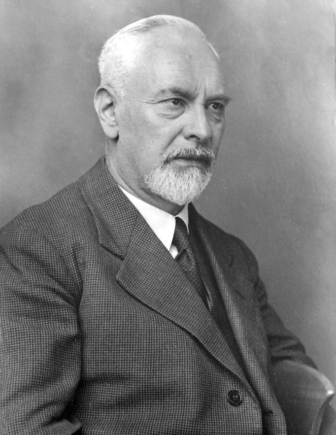
To set the stage for an exploration that will consume many columns to come, this installment will present some of the observations and follow many of the arguments gleaned from the article Ludwig Prandtl’s Boundary Layer by John D. Anderson Jr published in the December 2005 issue of Physics Today.
According to Anderson, Ludwig Prandtl
revolutionized fluid dynamics with a very simple to understand and yet highly non-intuitive concept of the boundary layer that exists in a fluid near a rigid surface.
To understand the importance of Prandtl’s result one has to start the story in the latter half of the 18th century, around the time Euler derived the ideal fluid equations bearing his name. The French mathematician Jean le Rond d’Alembert derived a paradox associated with ideal fluid flow. He proved that, for an incompressible fluid with no viscosity (i.e., an ideal fluid), the drag force on an object placed within this flow, moving with constant relative velocity with respect to the fluid, is identically zero, an obviously incorrect result.
Acheson presents a mathematical derivation of d’Alembert’s paradox In Section 4.13 of his book Elementary Fluid Dynamics. This derivation examines the force and momentum balance in the fluid and, using Bernoulli’s streamline theorem, concludes that, for the fluid to be moving at a uniform speed far upstream and far downstream from the body, the drag force on the body must vanish. This result contradicts everyday observations about the motion of solid objects in air or water.
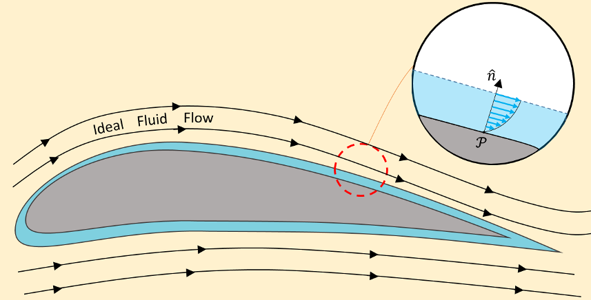
Clearly something was wrong with the theory of ideal fluid, but the specific root of the problem escaped identification for roughly 150 years until Prandtl introduced his boundary layer at a conference in 1904. The modern picture of the boundary layer is best understood in terms of the motion of air over a cambered wing as shown in the figure below (based on Figure 2 of Anderson).
Away from the wing, the ideal fluid model works well in describing the streamlines. However, close to the wing’s surface, viscous effects become dominant in a thin layer whose base attaches to the wing’s surface. This no-slip condition demands that the fluid be at rest at the surface and that the fluid velocity rapidly rise from zero (where the layer attaches to the wing) to the ‘free stream’ velocity of the bulk inviscid flow outside the layer (shown in the inset). In this way, d’Alembert’s paradox is conceptually resolved. The drag force is non-zero, as observed, and the bulk flow is inviscid or ideal (depending on whether one allows the viscosity-free flow to be compressible or not), as observed, but the mathematical conditions by which d’Alembert derived the paradox are not true everywhere – the thin boundary layer makes all the difference.
Prandtl also predicted that, in certain cases, this layer can separate from the surface, which can cause additional drag. To quote Prandtl
…there ought to be a layer of fluid which, having been set in rotation by the friction on the wall, insinuates itself into the free fluid, transforming completely the motion of the latter, and therefore playing there the same part as the Helmholtz surfaces of discontinuity.
Indeed, modern theory classifies the boundary layer behavior as falling into two broad classes. Laminar motion describes the flow when the layer stays fixed to the surface. Turbulent motion describes the flow when the layer separates and produces vortices in wake. Laminar flow produces less drag than turbulent flow but it is unstable and thus harder to produce or control. Turbulence changes the characteristics of the flow far from the surface causing additional drag.
In addition to these two critical physical observations, Anderson points out that the concept of the boundary layer also enabled the first quantitative calculations of aerodynamic drag. The reason for this is that the boundary layer equations exhibit an entirely different type of mathematical behaviors than the equations describing the bulk flow outside. Although both sets of equations are coupled, nonlinear, partial differential equations, the Navier-Stokes equations used to describe the bulk flow external to the layer are elliptic (at least when the flow is subsonic) while the simplification of these equations in the boundary layer are parabolic. This distinction allows the solution methods used to describe the bulk motion to ‘decoupled’ from the methods used to describe the drag and since the methods for solving parabolic equations are much easier to deal with than those for elliptic equations real progress can be made.
What is particularly amazing about Prandtl’s contribution is that the original presentation in 1904 lasted no longer than 10 minutes. I would say that the return on investment resulting from that rather short talk have been nothing short of phenomenal.
One of the more difficult things for any student of fluid dynamics to understand is the distinction between streamlines and streaklines and pathlines. It ranks up there with mastering the difference between the Eulerian and Lagrangian viewpoints and, in fact, the same difficulty underpins both – the ability to tell the difference between an attribute of the field (Eulerian point-of-view) and an attribute of the particle or fluid element (Lagrangian point-of-view). And, I’ll confess, that even though I understand the definitions, it isn’t always obvious how to apply them in different contexts.
Wikipedia has a somewhat useful article on the distinction between streamlines, streaklines, and pathlines but the math presented obscures the underlying physics and the foundation (either directly or by reference) is sorely lacking.
The first thing to note is that if the flow is steady, then all three lines result in the same trace in the fluid. This is because each fluid element, flowing through a given point, follows exactly the same trajectory as the fluid element that precedes it or follows it. The distinction between these lines (and possibly a few more differently defined traces) comes when the flow is unsteady (varies in time).
The formal definitions of these lines is as follows:
Streamline – a trace formed so that it is everywhere tangent to the velocity field of some local region of the fluid at a given time
Streakline – a trace of the front of all fluid elements, at a given time, that originated from the same physical place (for example a nozzle that flows smoke into a wind tunnel)
Pathline – a trace of the motion through time of a particular fluid element
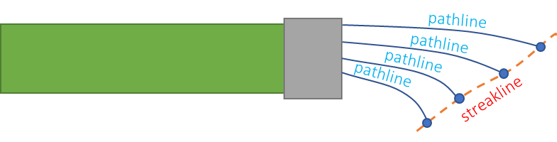
These formal definitions don’t do a lot to promote understanding the situation. So, we turn to an introductory diagram to explain the difference between streakline and pathline (streamlines will be discussed below) and then we will look at a simple example of unsteady flow to see the mathematical difference of all three.
Consider fluid starting to come out of a garden hose as the faucet is turned on. The flow may start weakly and then climb until it levels off at the steady state value. Below is a diagram of such a situation (inspired by the lecture from the Cowan Academy). The individual pathlines are quite different and the time the fluid elements came through the outlet of the hose are different. But their motion is stopped at a common time and the line joining them is the streakline. It is particularly useful in that it represents an experiment that can be performed and measured.
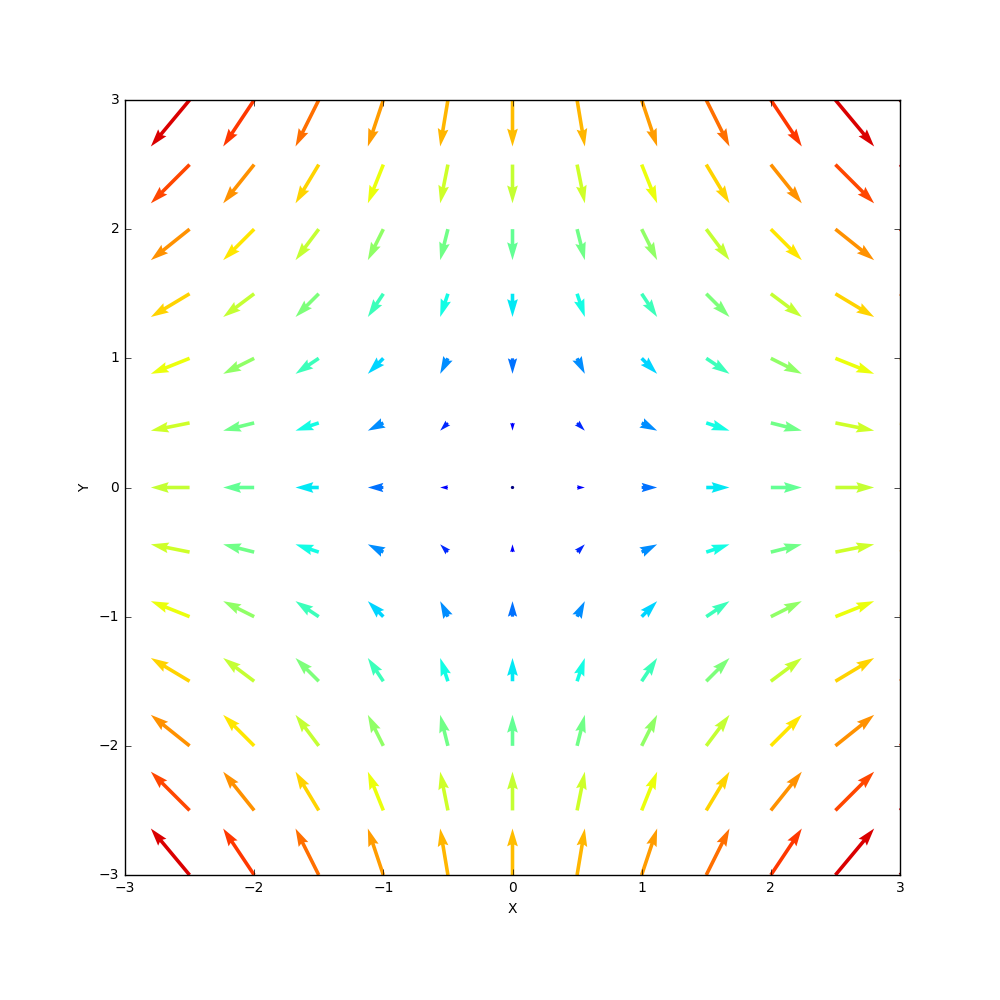
Streamlines are best shown using a quiver plot. To be concrete consider the velocity field in 2 dimensions to be given by
\[ V_x= \alpha x \; \]
and
\[ V_y = -\alpha y \; ,\]
where $$\alpha$$ is some real number. A plot of the flow velocity at a grid of points is called a quiver plot and the results for the flow above are (with $$\alpha = 1$$)
Note that the color of the vectors match their length with red corresponding the largest flow rate and blue the smallest, that they suggest that hyperbolic pattern with flow coming in along the y-axis and flowing along the x-axis, and the is a stagnation point at the origin where the fluid elements there are at rest.
Acheson, in Chapter 1 of Elementary Fluid Dynamics, has a nice problem associated with this flow that accentuates the difference between Lagrangian and Eulerian viewpoints. In the Eulerian viewpoint, the concentration of a pollutant is given by
\[ c(x,y,t) = \beta x^2 y e^{-\alpha t} \; ,\]
which clearly varies in space and time and fades in strength at a given point as time progresses. The question Acheson asks is does the concentration in a fluid element change. To answer, we employ the material derivative, since it follows the flow of a given material element. Taking the material derivative of the concentration gives
The right-hand side of the equation is a set of partial derivatives that, when expanded, is
\[ \partial_t c + \alpha x \partial_x c – \alpha y \partial_y c = -\alpha \beta x^2 y e^{-\alpha t} + 2 \alpha \beta x^2 y e^{-\alpha t} – \alpha \beta x^2 y e^{-\alpha t} = 0 \; . \]
So, the concentration of a fluid element is constant. The reason the concentration decays in strength at a given point is simply that the flow shunts the more polluted elements away from any point and towards infinity. Alternatively, one can use Lagrangian coordinates to describe the flow. The position of a given fluid element is given by
\[ x = X e^{\alpha t} \; \; y = Y e^{-\alpha t} \; , \]
where $$X$$ and $$Y$$ are the x- and y-position of the fluid element at $$t=0$$. In terms of these coordinates the concentration of a fluid element is
\[ c = \beta X^2 e^{-2 \alpha t} Y e^{\alpha t} e^{\alpha t} = \beta X^2 Y \; ,\]
which is manifestly time independent.
With this warm up exercise under our belt, let’s look at an unsteady flow where the difference between streamlines and pathlines becomes obvious.
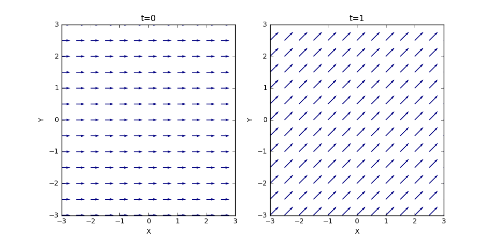
Consider the flow
\[ V_x = V_{x_0} \; \; V_y = k t \; \]
The quiver plots for two different times are shown here (with $$V_{x_0} = 1$$ and $$k=1$$).
In both cases, the streamlines are straight lines but with a time varying slope, as evidenced by the different slopes at different times.
The pathlines come from integrating
\[ \frac{\partial x}{\partial t} = V_{x_0} \;\; \textrm{and} \;\; \frac{\partial y}{\partial t} = k t \; .\]
Performing the integration and and setting the integration constants ($$x(t=0) = X$$ and $$y(t=0) = Y $$) to zero gives
\[ x(t) = V_{x_0} t \;\; \textrm{and} \;\; y(t) = \frac{1}{2} k t^2 \; .\]
Solving the first equation for $$t$$ and substituting into the second equation gives the geometric path of
\[ y = \frac{1}{2} \frac{k}{V_{x_0}^2} x^2 \; , \]
which shows that the particles follow a parabolic pathline even though the streamlines are always linear.