Monthly Archive: June 2015

This week the Lie series faces a stiff challenge in the form of the Kepler problem. Unlike some of the cases previously examined in this blog (harmonic oscillator, quantum wave propagation, etc.) the Kepler problem is nonlinear when written in the usual fashion in terms of Cartesian coordinates. There is a standard ‘clever’ substitution that make everything look linear ($$u = 1/r$$) but this won’t be employed.

In terms of the Cartesian coordinates, the orbital state for the Kepler problem is

\[ \bar s = \left[ \begin{array}{c} \vec r \\ \vec v \end{array} \right] \; ,\]

where $$\vec r$$ and $$\vec v$$ are the position and velocity of a reduced mass moving in a central potential $$V(r) = 1/r$$.

The equations of motion in state space notation are

\[ \frac{d}{dt} \bar S = \left[ \begin{array}{c} \vec v \\ -\frac{\mu \vec r}{r^3} \end{array} \right] \; ,\]

with initial conditions $$\vec r(t_0) = \vec \rho$$ and $$\vec v(t_0) = \vec \nu$$.

The corresponding Lie operator, which is written in terms of the initial conditions is

\[ D = \sum_i \nu_i \frac{\partial}{\partial \rho_i} – \frac{\mu \rho_i} {\rho^3} \frac{\partial}{\partial \nu_i } \; \]

or more compactly (with some slight abuse of notation)

\[ D = \vec \nu \cdot \partial_{\vec \rho} – \epsilon \vec \rho \cdot \partial_{\vec \nu} \; ,\]

where $$\epsilon = \mu/\rho^3$$ has been defined for future convenience.

The full solution is then given by the application of the Lie series operator $$L$$ to the initial position $$\vec \rho$$

\[ \vec r(t) = L[ \vec \rho ] \; .\]

With $$D$$ being nonlinear, the expansion implicit in this solution is very difficult to evaluate to all orders so a truncation of the expansion to order $$(t-t_0)^3$$

\[ L[\vec \rho] = e^{(t-t_0) D} \vec \rho \approx \left[ 1 + (t-t_0) D + \frac{ (t-t_0)^2}{2!} D^2 + \frac{(t-t_0)^3}{3!} D^3 \right] \vec \rho \]

will be employed with an eye for what patterns emerge.

A little bit of organization usually serves well in these types of expansions and, with that in mind, we note the following evaluations

\[ D \vec \rho = \vec \nu \; ,\]

\[ D^2 \vec \rho = D \vec \nu = – \frac{ \mu }{\rho^3} \vec \rho = – \epsilon \vec \rho \; ,\]

and

\[ D^3 \vec \rho = D( -\epsilon \vec \rho) = -\vec \nu \cdot \partial_{\vec \rho} \epsilon – \epsilon \vec \nu \; . \]

The third order expansion takes the form

\[ L[\vec \rho] \approx \vec \rho + (t-t_0) \vec \nu – \frac{ (t-t_0)^2 }{2!} \epsilon \vec \rho – \frac{ (t-t_0)^3 }{3!} \left( \vec \nu \cdot \partial_{\vec \rho} \epsilon + \epsilon \vec \nu \right) \; .\]

The last remaining partial derivative evaluates to

\[ \vec \nu \cdot \partial_{\vec \rho} \epsilon = \vec \nu \cdot \partial_{\vec \rho} \frac{\mu}{\rho^3} = -\frac{3 \vec \nu \cdot \vec \rho \mu}{\rho^5} \; . \]

Defining one last ‘greek’ shorthand (the reason for this will emerge shortly)

\[ \lambda = \frac{\vec \nu \cdot \vec \rho}{\rho^2} \]

allows the expansion to take the form

\[ L[\rho] \approx \vec \rho + (t-t_0) \vec \nu – \frac{ (t-t_0)^2 }{2!} \epsilon \vec \rho – \frac{ (t-t_0)^3 }{3!} \left( 3 \epsilon \lambda \vec \rho – \epsilon \vec \nu \right) \; .\]

What to make of this expansion? Compare this against the Taylor’s series expansion of the position (see ‘An Introduction to the Mathematics and Methods of Astrodynamics, Revised Edition’ by Battin, pp 110-112)

\[ \vec r(t) = \vec r0 + (t-t0) \left . \frac{d \vec r}{dt} \right|_{t=t0} + \frac{(t-t0)^2}{2!} \left. \frac{d^2 \vec r}{d t^2} \right|_{t=t0} \\ + \frac{(t-t0)^3}{3!} \left. \frac{d^3 \vec r}{d t^3} \right|_{t=t0} + \cdots \; .\]

Apparently, Lagrange defined the following ‘invariants’ (there are three of them but I’m only using the first 2)

\[ \epsilon = \frac{\mu}{r^3} \]

and

\[ \lambda = \frac{ \vec r \cdot \vec v }{ r^2 } \; \]

In terms of these classical invariants, the first three derivatives in the Taylors series become

\[ \frac{d \vec r}{dt} = \vec v \; , \]

\[ \frac{d^2 \vec r}{dt^2} = -\epsilon \vec r \; ,\]

and

\[ \frac{d^3 \vec r}{dt^3} = 3 \epsilon \lambda \vec r – \epsilon \vec v \; .\]

The series expansion thus agrees with the Lie series method or, in other words, the Lie series has reproduced the classical Lagrange f-g series

\[ \vec r(t) = f(t) \vec \rho + g(t) \vec \nu \; .\]

While there is really no new content that the Lie series has provided it does provide a few advantages. The first is that the notation is much more compact than the traditional approach using the Lagrange invariants. Second, the Lie series is clearly extensible to other, more complex problems and in such a fashion that is seems to provide a theoretical insight.

I’ll try to flesh this idea out next week when I apply the Lie series to the pendulum problem.

This column, which is a relatively short one as I am still grappling with the details, is the introductory piece for what I intend to be a through exploration of the use of Lie Series as a method for solving differential equations. This particular entry is heavily influenced by the NASA Technical Note TN D-4460 entitled ‘On the Application of Lie-Series to the Problems of Celestial Mechanics’ by Karl Stumpff, dated June 1968.

Stumpff starts his note with the following interesting passage:

That passage is interesting mostly due what the meaning of ‘Recently’ is. In his references, Stumpff lists only one work by Grobner, entitled “Die Lie-Reihen und ihre Anwendungen” dated 1960. Sophus Lie, from whom the Lie series derives it’s name, died in 1899 and it seems that it took 61 years for his work to really penetrate celestial mechanics.

The central idea of the Lie series is the production of an operator that makes the solution of certain differential equations manifest and their expansion in terms of a power series ‘automatic’. In presenting the prescription, I follow Stumpff’s ordering closely but with modifications of the notation to suit my tastes and needs.

Assume that there are $$n$$ functions

\[ F_i(z) = F_i(z_1, z_2, \dots, z_n) \]

in $$n$$ complex variables $$z_i$$ that are analytic in the neighborhood of

\[ \zeta = (\zeta_1, \zeta_2, \dots, \zeta_n) \; . \]

The concept of a Lie series depends on first defining the operator

\[ D = F_1(z) \frac{\partial}{\partial z_1} + F_2(z) \frac{\partial}{\partial z_2} + \dots + F_n(z) \frac{\partial}{\partial z_n} \; .\]

The operator $$D$$ is a derivation. That is to say it obeys the following properties.

It is linear

\[ D[f(z) + g(z) ] = D[f(z)] + D[g(z)] \; ,\]

it operation on a constant results in zero

\[ D[ c f(z) ] = c D f(z) \; , \]

and it obeys the Liebniz rule

\[ D[f(z) g(z) ] = f(z) \cdot Dg(z) + Df(z) \cdot g(z) \; .\]

Repeated application of the $$D$$ operator on the product of two functions results in the usual binomial expansion

\[ D^n [ f(z) g(z) ] = \sum_{\nu = 0}^{n} \left( \begin{array}{c} n \\ \nu \end{array} \right) D^{\nu} f(z) D^{n-\nu} g(z) \; .\]

Now the Lie series operator $$L$$ is defined as

\[ L(z,t) f(z) = e^{t D} f(z) \; , \]

where the exponential notation is short-hand for the series

\[ L(z,t) f(z) = \sum_{n=0}^{\infty} \frac{t^n}{n!} D^n f(z) = \left[1 + t D + \frac{t^2}{2!} D^2 + \dots \right] f(z) \; .\]

Note that often, the arguments $$(z,t)$$ are omitted.

Now an interesting and useful property of the Lie series operator for the product of two functions is

\[ L[f(z)g(z)] = L[f(z)] \cdot L[g(z)] \; ,\]

or in words, that the Lie series of a product is the product of the Lie series. This relationship is called the interchange relation.

Since we imagine that all the functions of interest are analytic, this simple relation ‘bootstraps’ to the general relation

\[ L[ Q(z)] = Q(L[z]) \; ,\]

for $$Q(z)$$ analytic.

As an example of this bootstrap relation, consider $$D = \frac{d}{dz}$$, and note that

\[ D^n[z] = 1 \delta_{n0} \]

and therefore

\[ L[z] = e^{t D}z = (1+ tD)z = z + t \; .\]

So the bootstrap relation gives first

\[ L[ Q(z)] = \sum_{n=0}^{\infty} \frac{t^n}{n!} \frac{d}{dz} Q(z) \; ,\]

which from elementary calculus is recognized to be $$Q(z+t)$$ expanded about $$t=0$$, and second

\[ Q(L[z]) = Q(z+t) \; . \]

Now the utility of the Lie series is not that it provides a compact way of representing a Taylor’s series (as convenient as that is) but rather in the fact that when the $$F_i$$ are not trivial functions it encodes solutions to a coupled set of differential equations. To see how this works, assume a system of differential equations given by

\[ \frac{d z_i}{dt} = F_i(z) \]

with initial conditions

\[ z_i(0) = \zeta_i \; .\]

Then the solution of this system of equations is

\[ z_i(t) = e^{t D} \zeta_i \; . \]

To see this, take the derivative of the solution to get

\[ \frac{d z_i(t)}{d t} = \frac{d}{dt} e^{tD} \zeta_i = D e^{t D} \zeta_i \; . \]

But, by definition, $$ e^{t D} \zeta_i = z_i(t) $$, so

\[ \frac{d z_i(t)}{d t} = D z_i = F_i \; . \]

In some sense, this is our old friend the propagator or state transition matrix written in a new form. However, this new encoding works for non-linear systems as well, a point that makes it an improvement on those approaches.

One last note. So far, the system of differential equations was assumed to be autonomous. In the event the system isn’t, a simple ‘trick’ can be used to make it look autonomous. Define a new variable $$z_0 = t$$ and the augment the definition of $$D$$ to be

\[ D = \frac{\partial}{\partial z_0} + \sum_{i=0}^{n} F_i(z) \frac{\partial}{\partial z_i} \; .\]

This manipulation has the advantage of making an non-autonomous system look formally autonomous. The only disadvantage is that all notion of equilibrium points are lost since the right-hand side of the equations can never have well-defined critical points.

Next time, I’ll apply the Lie series formalism to the Kepler problem

Last week, we discussed how a clever interrogation of the Maxwell’s equations to find a variety of relations, including the derivation of Poynting’s theorem. This week, I thought it would be interesting to look a little more at how the Poynting’s theorem works for a set of special cases.

The first case looks at the propagation of the an electromagnetic wave. In this case, common intuition as to the direction of the energy flow will match the mathematics and all looks right with the world. The second case involves a uniform current is put through a resistive wire. This common situation ends up an unusual interpretation of the Poynting flux. The third case, which involves running AC current through a capacitor in a circuit, common intuition about the direction of $$\vec S$$ turns out to be quite wrong and the result is both puzzling and instructive.

On note, before the dissection of the two cases begins. This post is heavily influenced by Chapter 10 in Electromagnetic Theory by Frankl and the discussion in Chapter 27 of the Feynman Lectures on Physics.

Case 1 – Propagation of an Electromagnetic Wave

One of the most celebrated results of Maxwell’s synthesis of the equations that bear his name and which follows from and, in some sense, motivated his inclusion of the displacement term in Ampere’s law is the prediction of electromagnetic waves. From the basic equations, a plane electromagnetic wave of frequency $$\omega$$ propagating in the $$k$$-direction (which can point anywhere) is described by

\[ \vec E(z,t) = \vec E_0 e^{i(\vec k \cdot \vec r – \omega t)} \]

for the electric field and by

\[ \vec B(z,t) = \vec B_0 e^{i(\vec k \cdot \vec r – \omega t)} \]

for the magnetic field.

Note that this form assumes that the wave propagates in free space and, therefore, doesn’t interact with matter. Applying Coulomb’s law ($$div(\vec E) = 0$$) gives

\[ \nabla \cdot \vec E = 0 \Rightarrow \vec E_0 \cdot \vec k = 0 \; .\]

Likewise, the application of the Monopole law leads to $$\vec B_0 \cdot \vec k = 0$$. So the electric and magnetic fields are perpendicular to the direction of propagation and since $$\vec S = \vec E \times \vec B / \mu_0$$ the Poynting flux is parallel to $$\vec k$$ just as common intuition indicates. The energy flow is along the direction of propagation.

Note that a careful computation will show that the magnitude of the energy flow is just what elementary wave mechanics would predict.

Case 2 – Current Through a Resistive Wire

In this case, a long straight wire with conductivity $$g$$ carries a current $$I$$ uniformly distributed across it. The relevant geometry is shown in the figure.

The current density is

\[ \vec J = \frac{I}{\pi a^2} \hat z \; .\]

The electric field needed to drive this current is

\[ \vec E = I R \hat z = I \frac{1}{\pi a^2 g} \hat z \]

and the resulting magnetic field set up by the current (by applying Ampere’s law) is

\[\vec H = \left\{ \begin{array}{c} \frac{I \rho}{2 \pi a^2 } \hat \phi \; \; \text{for} \; \; \rho < a \\ \frac{I}{2 \pi \rho} \hat \phi \; \; \text{for} \; \; \rho >a \end{array} \right. \; , \]

where $$\hat \phi$$ is the unit vector pointing along the azimuthal angle direction and $$\hat \rho$$ points along the radial direction in cylindrical coordinates (i.e. both are confined to the $$x$$-$$y$$ plane in cylindrical coordinates). The Poynting vector evaluates to

\[\vec S = \left\{ \begin{array}{c} -\frac{I^2 R}{2 \pi} \frac{\rho}{a^2} \hat \rho \; \; \text{for} \; \; \rho < a \\ - \frac{I^2 R}{2 \pi} \frac{1}{\rho} \hat \rho \; \; \text{for} \; \; \rho > a \end{array} \right. \; .\]

Note the peculiar nature of the direction of the energy flow. It isn’t along the wire but radially in from the outside.

Now a concern may be raised that there is an error somewhere hidden in the manipulations up to date. To assuage these concerns and build confidence, compute the divergence of the Poynting vector. The result should be related to the energy dissipation happening due to the resistance. The divergence is (recall that, in cylindrical coordinates, $$\nabla \cdot (A_{\rho} \hat \rho) = \frac{1}{\rho} \partial_{\rho} (\rho A_{\rho})$$) :

\[\nabla \cdot \vec S = \left\{ \begin{array}{c} -\frac{I^2 R}{\pi a^2} \; \; \text{for} \; \; \rho < a \\ 0 \; \; \text{for} \; \; \rho > a\end{array} \right. \; . \]

The dissipation within the wire is given by

\[ \vec E \cdot \vec J = \frac{I^2 R}{\pi a^2} \; ,\]

and the Poynting theorem is

\[ \nabla \cdot \vec S + \partial_t u = – \vec E \cdot \vec J \; .\]

Since the situation is static, all partial time derivatives are zero and we should see that $$\nabla \cdot \vec S = – \vec E \cdot \vec J$$, which happily is the result. So, despite what may seem to fly in the face of intuition, the theory holds together.

Case 3 – Run AC Current Through a Capacitor

This case is an intermediate case between the previous two, in which a low-frequency current is driven through a capacitor. This situation is intermediate between the first two – it does not involve static fields but does confine the action to a local circuit element. The relevant geometry is shown in the following figure.

Assuming that the frequency is small enough to ignore the energy in the magnetic field, the total energy contained between the plates is

\[ U_{tot} = u \cdot Vol = (\frac{1}{2} \epsilon_0 E^2)(\pi a^2 h) \]

and it changes as function of time as

\[ \partial_t U_{tot} = \epsilon_0 \pi a^2 h E \partial_t E \; .\]

From an application of Ampere’s law applied to the surfaces of the capacitor, converting the surface integral over $$curl(\vec B)$$ to a line integral along the boundary and using $$\mu_0 \epsilon_0 = 1/c^2$$, yields

\[ 2 \pi a c^2 B = \partial_t E \pi a^2 \; ,\]

which solved for $B$ gives

\[ B = \frac{a}{2 c^2} \partial_t E \; .\]

The direction of $$\vec E$$ is along the axial direction of the capacitor and the direction of $$\vec B$$ is azimuthal. From these facts, it is obvious that the Poynting vector must be pointing radially inward, as shown in the figure.

The magnitude of the Poynting vector is (note the simplification since the electric and magnetic field are perpendicular)

\[ |\vec S| = |\vec E| |\vec B| =\frac{1}{\mu_0} E \frac{a}{2 c^2} \partial_t E = \frac{1}{2} \epsilon_0 a E \partial_t E \; . \]

The total energy flow in is given by the product of the magnitude of the Poynting vector times the total surface area

\[ \Delta U = |\vec S| \cdot Area = (\frac{1}{2} \epsilon_0 a E \partial_t E) (2 \pi a h) = \epsilon_0 \pi a^2 h E \partial_t E \; , \]

which is happily the same result we got above.

So once again, the flow of the energy seems counterintuitive but the results that follow agree with what is expected.

One of the more fun things to do with physical models is to mine general results without actually solving specific problems. Its fun because it is relatively easy to do and gives some global insight into the problem that is not easily obtainable from examining individual cases. Usually, this type of data mining comes from considerations of symmetry or general principles and takes the form of clever manipulations of the underlying equations. Like any good riddle, the joy is in seeing the solution – the frustration is in trying to find it for the first time.

Of course, to find these nuggets of general fact, one needs to know, or at least firmly believe, they are there. Conservation laws for energy, momentum, and angular momentum are cherished principles that took many decades to be ferreted out of many specific cases.

Nonetheless, we can all stand on the shoulders of giants and enjoy the view and that is what this post is all about. Standing on the shoulders of Maxwell, one can mine the equations that bear his name for all sorts of nuggets.

The version of Maxwell’s equations that I’ll use describes the behavior of the macroscopic fields with the appropriate constitutive equations. These are:
\[ \nabla \times \vec H = \vec J + \frac{\partial \vec D}{\partial t} \; , \]
\[ \nabla \times \vec E = -\frac{\partial \vec B}{\partial t} \; ,\]
\[ \nabla \cdot \vec D = \rho \; ,\]
and
\[ \nabla \cdot \vec B = 0 \; , \]
as the differential expressions for Ampere’s, Faraday’s, Coulomb’s and the Monopole’s laws.

Since dimensional analysis will be important below, note that fields and sources have units of

• $$\vec E$$ – $$[N/C]$$ or $$[V/m]$$
• $$\vec D$$ – $$[C/m^2]$$
• $$\vec B$$ – $$[Ns/Cm]$$ or $$[kg/Cs]$$
• $$\vec H$$ – $$[A/m]$$
• $$\vec J$$ – $$[C/m^2/s]$$
• $$\rho$$ – $$[C/m^3]$$
• $$\epsilon$$ – $$[C^2/Nm]$$
• $$\mu$$ – $$[N/A^2]$$

There are three very nice interrogations of these laws that yield: 1) charge conservation, 2) energy and momentum conservation (in the absence of external forces), and 3) the guarantee that a solution to the initial value problem (Coulomb and monopole equations) is preserved by the propagation of the system forward in time. This latter property will be called constraint preservation.

Charge Conservation

As they appear in their usual form, the Maxwell equations don’t immediately show that they honor the conservation of charge. That they actually do is seen by first starting with Ampere’s law and take the divergence of both sides to get

\[ \nabla \cdot \left( \nabla \times \vec H = \vec J + \frac{\partial \vec D}{\partial t} \right ) \Rightarrow \nabla \cdot \nabla \times \vec H = \nabla \cdot \vec J + \nabla \cdot \frac{\partial \vec D}{\partial t} \; . \]

Since the divergence of a curl is zero, the left-hand side disappears. Next interchange of the divergence operator with the partial derivative with respect to time, $$\partial_t$$ to get

\[ 0 = \nabla \cdot \vec J + \frac{\partial ( \nabla \cdot \vec D )}{\partial t} \; . \]

Now the last term on the right-hand side can be put into familiar form by using Coulomb’s law and, with one more minor manipulation, yields the familiar form of the charge conservation law

\[ \nabla \cdot \vec J + \frac{\partial \rho}{\partial t} = 0 \; .\]

Energy and Momentum Conservation

The starting point for this conservation is the proof of the Poynting theorem. Form the dot product between $$\vec H$$ and both sides of Faraday’s law to get

\[ \vec H \cdot \nabla \times \vec E = – \vec H \cdot \partial_t \vec B \]

Rewrite the left-hand side using the vector identity

\[ \nabla \cdot (\vec A \times \vec B) = (\nabla \times \vec A) \cdot \vec B – \vec A \cdot (\nabla \times \vec B) \]

giving

\[ \nabla( \vec E \times \vec H ) + \vec E \times (\nabla \times \vec H) = – \vec H \cdot \partial_t \vec B \]

Now use Ampere’s law to substitute for $$\nabla \times H $$, yielding

\[ \nabla( \vec E \times \vec H ) + \vec E \times (\vec J + \partial_t \vec D) = – \vec H \cdot \partial_t \vec B \]

which, when rearranged, gives the Poynting theorem

\[ \nabla \cdot (\vec E \times \vec H ) + \vec H \cdot \partial_t \vec B + \vec E \cdot \partial_t \vec D = – \vec E \cdot \vec J \]

Make the following identifications

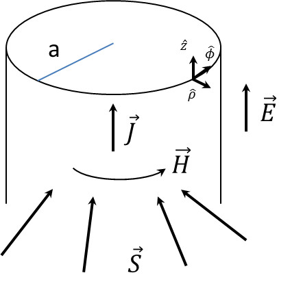
\[ \vec S = \vec E \times \vec H \]

and

\[ u = \frac{1}{2} \left( \vec E \cdot \vec D + \vec H \cdot \vec B \right) \]

to get the common form of

\[ \nabla \cdot \vec S + \partial_t u = – \vec E \cdot \vec J \]

for Poynting’s theorem.

Now for some dimensional analysis. The quantities $$u$$, $$\vec S$$, $$\vec E \cdot \vec J$$, $$\nabla \cdot \vec S$$, and $$\partial_t u$$ have units of:

• $$u$$ – $$[N/C][C/m^2] + [Ns/Cm][C/sm]=[N/m^2] = [J/m^3]$$
• $$\vec S$$ – $$[N/C][C/sm] = [N/ms] = [Nm/m^2s] = [J/m^2s]$$
• $$\vec E \cdot \vec J$$ – $$[N/C][C/m^2s]=[Nm/m^3s] = [J/m^3s]$$
• $$\nabla \cdot \vec S $$ – $$[N/m^2s] = [Nm/m^3s] = [J/m^3s]$$
• $$\partial_t u$$ – $$[J/m^3][1/s] = [J/m^3s]$$

The obvious interpretation is that $$u$$ is an energy density, $$\vec S$$ is the energy flow (flux) and the $$\vec E \cdot \vec J$$ is the work done on the charges by the electric field per unit volume (power density).

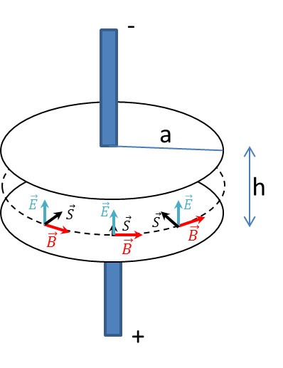
There is a way to connect the Poynting theorem to momentum since photons obey $$E^2 = c^2 \vec p^2$$. For simplicity, the expression of the Poynting vector in free space and in terms of the magnetic permeability $$\mu_0$$ and the magnetic flux density $$\vec B$$ is

\[ \vec S = \frac{1}{\mu_0} \vec E \times \vec B \; .\]

A check of the Poynting vector units from the definition to find $$\underbrace{ [A^2/N] }_{1/\mu_0} \underbrace{ [N/C] }_{\vec E} \underbrace{ [Ns/Cm] }_{\vec B} = [N/ms]$$. Now these unit can be put into a more suggestive form as either $$[N/ms] = [Nm/m^3][m/s] = [J/m^3][m/s]$$, which suggests interpreting the Poynting vector as a energy density times a speed or as $$[N/ms] = [Nm][1/m^2/s] = [J/m^2/s] = [J/s/m^2] = [W/m^2]$$, which represents a power flux.

So dividing by the speed of light, in the appropriate form, gives

\[ \frac{1}{c} \vec S = \sqrt{ \frac{\epsilon_0}{\mu_0} } \vec E \times \vec B = \sqrt{ \epsilon_0 \mu_0 } \vec E \times \vec H \]

which represents either a momentum flux or a momentum density times speed. Since $$\vec S/c$$ has units of momentum density times speed one may guess that $$\vec S/c^2$$ is the field momentum density. This is true even in the presence of matter allowing the general definition of

\[ \frac{1}{c^2} \vec S = \underbrace{ \mu \epsilon \vec E \times \vec H}_{\text{field momentum density}} \; .\]

Frankl, in his Electromagnetic Theory (pp. 203-4), presents a nice argument, based on the Lorentz force law, to relate the field momentum to the particle momentum to show that

\[ \vec F_{total} = \frac{d}{dt}\left[ \vec p_{particles} + \int d^3 r \, \mu \epsilon \vec E \times \vec H \right] \; .\]

To see this, start with the Lorentz force law ($$\vec F = q (\vec E + \vec v \times \vec B)$$) expressed in terms of particle and field densities using Ampere’s and Coloumb’s laws

\[ \vec f = \rho \vec E + \vec J \times \vec B = (\nabla \cdot \vec D) \vec E – \vec B \times (\nabla \times \vec H) – \partial_t \vec D \times \vec B \; .\]

Using the Faraday and Monopole laws gives

\[ 0 = – \vec D \times (\nabla \times \vec E) – \vec D \times \partial_t \vec B \]

and

\[ 0 = – \vec H \, \nabla \cdot \vec B \; .\]

Adding the above relations to the Lorentz force law relation gives

\[ \vec f = \epsilon ( \vec E \, \nabla \cdot \vec E – \vec E \times (\nabla \times \vec E) ) + \mu ( \vec H \, \nabla \cdot \vec H – \vec H \times ( \nabla \times \vec H ) ) – \mu \epsilon \, \partial_t ( \vec E \times \vec H ) \; .\]

Integrate over all space using the identity

\[ \int d^3r \, (\vec G \nabla \cdot \vec G – \vec G \times \nabla \times \vec G) = \int d^2S \left( \vec G (\vec G \cdot \hat n) – \frac{1}{2} G^2 \hat n \right) \]

that allows two of the volume integrals to become surface integrals resulting in

\[ \underbrace{ \frac{d}{dt} \vec p_{particles} }_{\vec F_{particles}} = I_{\vec E} + I_{\vec H} – \frac{d}{dt} \int d^3r \, \mu \epsilon \vec E \times \vec H \; .\]

Finally, Frankl attaches meaning to the surface integrals by first looking at the situation where the fields are static to pick out the total force as

\[ \frac{d}{dt} \vec p_{particles} = \underbrace{ I_{\vec E} + I_{\vec H} }_{\text{total force}} \; .\]

Since the instantaneous configuration of the fields and the particles cannot ‘know’ the future, $$I_{\vec E} + I_{\vec H}$$ must always be the total force. Bring the field piece over to the left hand side gives

\[ \frac{d}{dt} \vec p_{particles} + \frac{d}{dt} \int d^3r \, \mu \epsilon \vec E \times \vec H = \underbrace{ I_{\vec E} + I_{\vec H} }_{\text{total force}} \; , \]

which suggests the identification of the field momentum as

\[ \vec p_{field} = \int d^3r \, \mu \epsilon \vec E \times \vec H \; ,\]

which is exactly the interpretation obtained above for the Poynting vector divided by the speed of light squared.

Now if the system is defined in such a way to be closed so that the electric and magnetic fields are zero on the boundary, then momentum and energy cannot flow out of the system and thus are conserved. Energy and momentum do flow between the particles and the fields, with one component gaining or losing as the other loses or gains, but never does any of the energy or momentum vanish.

Constraint Preservation

The two Maxwell equations involving the curl operator are dynamical – that is to say that the spatial derivatives are tied to derivatives with respect to time. The two Maxwell equations involving the divergence operator involve no time derivatives. This latter two are interpreted as constraint equations that the field must satisfy at each time step. The operative question is if the fields satisfy these constraints at some initial time, if the subsequent propagation of the field forward in time, described by the dynamical equations, really honors the constraints. That is to say, that the constraints will continue to be satisfied. This is a very important point, as any theory that fails to keep the constraints satisfied is physically untenable. To check whether Maxwell’s equations do preserve these constraints, start by taking the divergence of Ampere’s equation as in the charge conservation case above

\[ \nabla \cdot \vec J + \partial_{t} (\nabla \cdot \vec D ) = 0 \; .\]

This time, instead of hunting for charge conservation, we are going to use charge conservation to eliminate $$div(\vec J)$$ in favor of $$\partial_t \rho$$ to get

\[ -\partial_t \rho + \partial_t (\nabla \cdot \vec D) = 0 \Rightarrow \partial_t (\nabla \cdot \vec D – \rho ) = 0 \; .\]

Note that a logical purist may object that this constraint and charge conservation are really not independent of each other and that this ‘proof’ is merely a tautology. This is actually true but is not a flaw. It simply means that charge conservation and the preservation of the Coulomb go hand-in-hand.

Likewise, taking the divergence of Faraday’s law gives

\[ \nabla \cdot (\nabla \times \vec E + \partial_t \vec B = 0 ) \; , \]

which because of the divergence of the curl is zero becomes

\[ \partial_t (\nabla \cdot \vec B = 0 ) = 0 \; ,\]

assuming that $$\partial_t$$ commutes with $$\nabla \cdot$$.

Thus, once both Coulomb’s Law and the Monopole Law are satisfied at at the initial conditions, they stay satisfied for all time.