The previous five columns have dealt with the Laplace Transform in detail, focusing on the basic properties and fundamental theorems. The applications to differential equations has been covered in passing with the exception of the one column that covered the application to the simple harmonic oscillator. That column showed the utility of the method but didn’t generalize to arbitrary state space dimensions. This shortcoming is easily overcome since the generalization is fairly obvious and easy. More critical is the inherent limitation of the Laplace Transform to linear systems and the ends to which the typical controls engineer goes to transform general problems to linear ones. It is to this last topic that this current column is devoted.
The basic approach of the controls engineer is to first express the dynamics of the system being modeled in state space form where the equation of motion is given by
\[ \frac{d}{dt} \bar S(t) = \bar f(t,\bar S) \]
where the state $$\bar S$$ is constructed so that any derivatives in the original model are replaced by auxiliary variables; for example $$v_x \equiv \dot x$$. Usually, the state variables are presented in column-array fashion. The right-hand side $$\bar f$$ contains the generalized form for the time derivatives of the state variables as governed either by the kinematic definitions (e.g. $$\dot x = v_x$$) or the dynamic relations (e.g. $$\dot v_x = f_x/m$$, where $$f_x$$ is the x-component of the force) and is, likewise, presented as a column array. Typically, the equations of motion possess a non-linear right-hand side, meaning that at least one component of $$\bar f$$ is a non-linear function of the state variables.
There are really two distinct but related ideas behind linearization. The first is the notion that the nonlinear functions in $$\bar f$$ can be replaced by linear approximations. The second is the idea of linearizing about a known solution to the equations of motion.
The pendulum serves as the textbook example of what to do in the first case. As discussed in an earlier post, the equation of motion of the angle $$\theta$$ makes with respect to the vertical takes the form
\[ \ddot \theta + g \sin \theta = 0 \; .\]
This nonlinear ordinary differential equation is linearized by expanding the sine and keeping only the first order term resulting in the harmonic oscillator approximation
\[ \ddot \theta + g \theta = 0 \; .\]
It is well established that this approximation is adequate only when $$\theta$$ is small (for example: see Numerical Solutions of the Pendulum).
The second concept of linearization is more subtle and involves looking at how deviations to a nominal solution evolve in time. To implement this linearization, we imagine that a solution $$\bar S_{\bar f}(t;\bar S_0)$$ of the original system exists given the initial conditions $$\bar S_0$$. We further imagine that deviations from the solution arise either due to differences in the initial conditions or in the right-hand side of the differential equation.
Both of these differences are physically realizable and lead to different contributions to the linearization. Physically, uncertainty in the initial state arises due to measurement limitations, either inherent ones due to quantum effects, or due to a lack of knowledge based on limits in metrology. Uncertainties in the right-hand side are due to our limited ability to infer the forces acting in a physical system based solely on the observed motion.
In realistic systems, both differences are present but it is convenient to study the two contributions separately before combining. The categorization to describe these different ‘mix-and-match’ scenarios is:
- State variation – differences in evolution due to uncertainties in the initial conditions
- Model variation – differences in evolution due to differences in the right-hand side
- Total variation – differences in evolution due to contributions from both sources
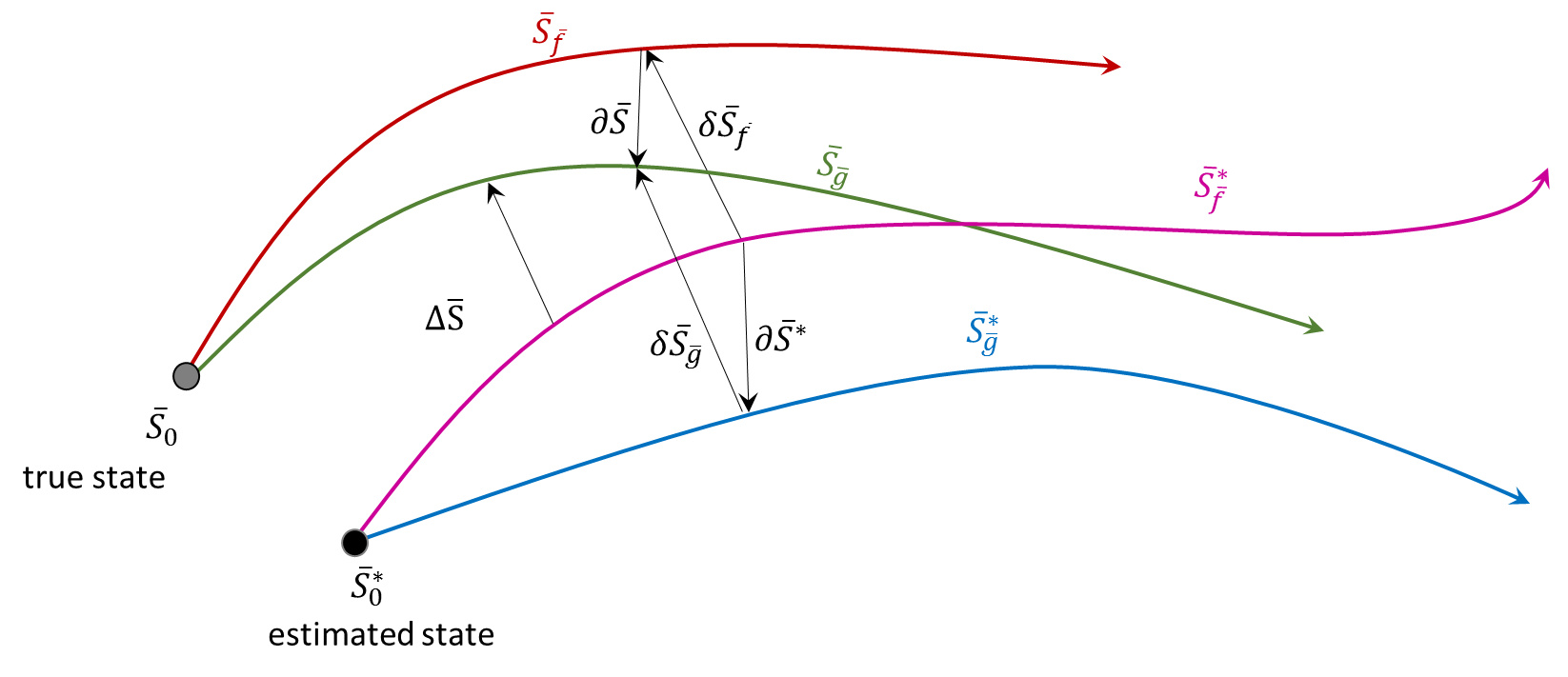
The following figure shows the evolution of two states, an estimated initial state $$\bar S^*_0$$ and a true initial state $$\bar S_0$$, each under the action of two right-hand sides $$\bar f$$ (estimated model) and $$\bar g$$ (true model). In this figure, $$\delta \bar S$$ is the state variation, $$\partial \bar S$$ is the model variation, $$\Delta \bar S$$ is the total variation.
The key assumption is that both the state and model variations lead to small deviations in the evolution. If this assumption holds, a linearized equation of motion for the state and total variations can be derived. Since the true state and model are not none for physical systems (as opposed to mathematical models) it is most useful to ultimately express all the deviations in terms of the state deviation under the estimated model, since this is the one most easily probed. The linearization is relatively easy and will be done for state and model variations first and then will be combined for the total variation.
State Variation
Start with the basic relation $$\delta \bar S = \bar S – \bar S^*$$. To calculate the differential equation for the state variation apply the time derivative to both sides
\[ \frac{d}{dt} \delta \bar S = \frac{d}{dt} \left[ \bar S – \bar S^* \right] \]
and use the original equation of motion to eliminate the derivatives of the state in favor of the right-hand sides of the differential equation.
\[ \frac{d}{dt} \delta \bar S = \bar f(\bar S) – \bar f (\bar S^*) \]
Since the model is the same in both cases, it really doesn’t matter which model is used but using $$\bar f$$ will be convenient later. Finally, express the true state in terms of the estimate state and the state deviation
\[ \frac{d}{dt} \delta \bar S = \bar f(\bar S^* + \delta \bar S) – \bar f(\bar S^*) \]
and expand
\[ \frac{d}{dt} \delta \bar S = \left. \frac{\partial \bar f}{\partial \bar S} \right|_{\bar S^*} \delta \bar S \; .\]
Note that the matrix $$A \equiv \left. \frac{\partial \bar f}{\partial \bar S} \right|_{\bar S^*}$$ is evaluated along the estimated trajectory (although in this case either will suffice) and is, in general, time-varying because of it.
Model Variation
The equation of motion for the model variation is the most analytically intractable of the variations and does not lead directly to a linear equation. To evaluate it, take the time derivative of the definition of the model variation
\[ \frac{d}{dt} \partial \bar S = \frac{d}{dt} \left[ \bar S_{\bar g} – \bar S_{\bar f} \right] \; . \]
Replace the derivatives on the right gives
\[ \frac{d}{dt} \partial \bar S = \bar g (\bar S) – \bar f(\bar S) \equiv \bar \eta_0(\bar S) \; .\]
This is as far as one can go with the general structure. But it is usually argued that if the actual forces are not producing a discernable signal (for if they were, they could be inferred from the motion) then $$\bar \eta_0$$ can be thought of as an inhomogeneous noise term. We will make such an argument and assume this property.
Total Variation
From the figure there are two equally valid definitions of the total variation in terms of true state
\[ \Delta \bar S = \delta \bar S_{\bar f} + \partial \bar S \]
and in terms of the estimated state
\[ \Delta \bar S = \delta \bar S_{\bar g} + \partial \bar S^* \; . \]
Equating, rearranging, and taking the time derivative yields
\[ \frac{d}{dt} \delta \bar S_{\bar g} = A \delta \bar S_{\bar f} – \bar \eta^*_0 – \bar \eta_0 \; \]
One last approximation is needed. Much like the argument above, it is based on a plausibility and not on a rigorous linearization. This argument says that if the differences between the two force models are small enough to regard the model variations to be noise-like, then for all practical considerations the state variations are approximately the same.
Thus the final equation is
\[ \frac{d}{dt} \delta \bar S_{\bar f} = A \delta \bar S_{\bar f} + \bar \eta \; \]
where $$\bar \eta$$ is a collected noise term (with an appropriate and insignificant sign change). It should be emphasized that this final equation is not rigorous correct but has been used by control engineers successful and so is worth studying.
