Monthly Archive: February 2016

The last post detailed how specific types of information could be gleaned from the equation of motion for a $$1/r$$ central potential. Three conserved quantities were discovered: the energy, the angular momentum, and the eccentricity vector. In addition, the radial equation, which gives the trajectory’s distance from the scattering center as a function of polar angle along the trajectory, presented itself after a clever manipulation.

This column presents specific techniques and results for modeling individual scattering trajectories for both repulsive ($$\alpha < 0 $$) and attractive ($$\alpha > 0$$) forces.

The first step in calculating specific, individual trajectories is the transformation of the equation of motion from the usual Newton form

\[ \ddot {\vec r} + \frac{\alpha \vec r}{r^3} = 0 \]

into a state space form. The most straightforward method is to use Cartesian coordinates, which yields the coupled first-order equations

\[ \frac{d}{dt} \left[ \begin{array}{c} x \\ y \\ z \\ v_x \\ v_y \\ v_z \end{array} \right] = \left[ \begin{array}{c} v_x \\ v_y \\ v_z \\ -\frac{\alpha x}{r^3} \\ -\frac{\alpha y}{r^3} \\ -\frac{\alpha z}{r^3} \end{array} \right] \; .\]

Numerical integration of the above system results in an ephemeris representation of the trajectory – a listing of discrete times and corresponding position components $$x, y, z$$ and velocity components $$v_x, v_y, v_z$$. Nonlinear combinations of the state will be used to determine the conserved quantities both as a check on the numerical method but also to emphasize the power affording by finding and exploiting conserved quantities.

All of the numerical modeling was done using Python 2.7, numpy, and scipy under the Jupyter notebook format. Matplotlib is used for all of the plots.

The core function used to integrate the equations of motion is

def TwoBody(state,t,params):
    #unpack the state
    x     = state[0]
    y     = state[1]
    z     = state[2]
    vx    = state[3]
    vy    = state[4]
    vz    = state[5]
    
    #unpack params
    alpha = params['alpha']
    
    #define helpers
    r     = sp.sqrt(x**2 + y**2 + z**2)
    q     = alpha/r**3
    
    #state derive
    ds = [vx, vy, vz, -q*x, -q*y, -q*z]
    return ds

Note its structural similarity to the coupled equation above – specifically, the function TwoBody returns the right-hand side of the system of differential equations. The scipy.integrate function odeint, which provides the numerical integration technique, takes this function, arrays specifying the initial conditions and the time span, and any additional arguments that need to be passed. In this case, the additional argument is a Python dictionary that contains the value of $$\alpha$$.

The odeint function returns an array of state values at the times contained in the array that specifies the time span. Together the two arrays comprise the ephemeris of the system.

One additional, useful ingredient is the function conserved_quantities

def conserved_quantities(soln,params):
    pos     = soln[:,0:3]
    vel     = soln[:,3:6]
    r       = np.sqrt((pos*pos).sum(axis=1)).reshape(-1,1) #makes the broadcast shape correct
    E       = 0.5*(vel*vel).sum(axis=1).reshape(-1,1) - params['alpha']/r #other reshape needed to avoid NxN shape for E
    L       = np.cross(pos,vel)
    Ecc     = np.cross(vel,L)/params['alpha'] -  pos/r
    return E, L, Ecc    

that takes the state array and returns arrays corresponding to the energy, the angular momentum vector, and the eccentricity vector. The conserved quantities serve two purposes. The first is that they help make sense out of the jumble of state variables. This was the point of last week’s column. The second is they provide indicators of the goodness of the numerical techniques. If they are not well conserved, then the numerical techniques are not doing what they should.

The first test case run was for the initial conditions

\[ \bar S_0 = \left[ \begin{array}{c} -30 \\ 0.1 \\ 0 \\ 2.25 \\ 0 \\ 0 \end{array} \right] \]

and a value of $$\alpha = -0.4$$. Since $$\alpha < 0 $$, the scattering is repulsive. The resulting trajectory is

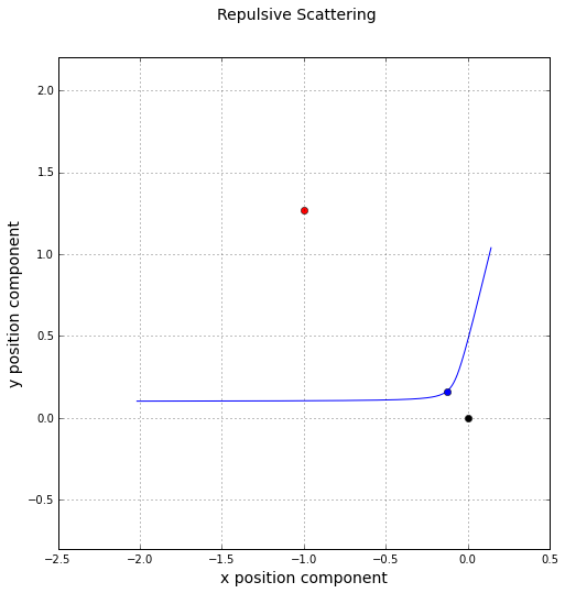
The black dot indicates the force or scattering center, the blue dot the point of closest approach, and the red dot location of the eccentricity vector.

While the trajectory looks like what we would expect, the is no obvious way to tell, from this figure, whether the ephemeris is correct. Based on the initial conditions, the conserved quantities should be

\[ E = 2.54458 \; ,\]

\[ \vec L = \left[ \begin{array}{c} 0 & 0 & -0.225 \end{array} \right]^T \; ,\]

and

\[ \vec E = \left[ \begin{array}{c} 1 & -1.268958 & 0 \end{array} \right]^T \; .\]

The figure below shows that error in each quantity, where the error is defined as the difference between the instantaneous value and the initial value (e.g. $$\epsilon_E = E(t) – E_0$$).

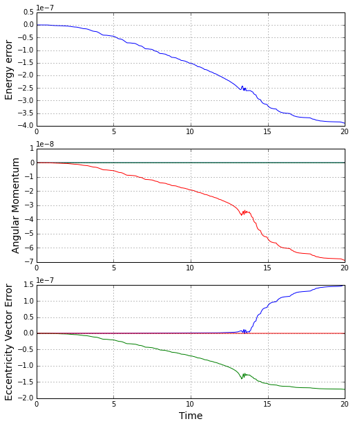
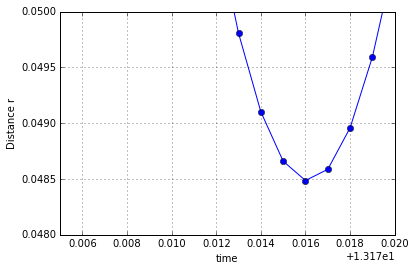
It is clear that the integration does an excellent job of honoring the conservation of the energy, angular momentum, and the eccentricity vector. So now we can believe that the ephemeris is accurate and can test the radial equation. The next figure shows the distance of the trajectory as a function of time in the neighborhood of the closest approach.

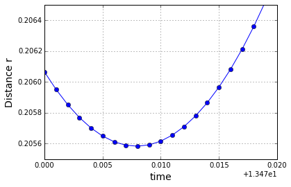
From the figure, the closest approach occurs at a distance of $$r = 0.2055838$$. The radial equation, which reads

\[ r(\nu) = \frac{L^2/|\alpha|}{e \cos\nu – 1} \; ,\]

predicts that the closest approach, which occurs at $$\nu = 0$$, of $$r_{CA} = \frac{L^2/|\alpha|}{e-1} = 0.2055838$$.

In the same fashion, we can generate a trajectory for $$\alpha = 0.4$$ with the same initial conditions as above. The resulting trajectory is

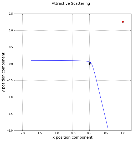
Based on the initial conditions, the conserved quantities should be

\[ E = 2.51792 \; ,\]

\[ \vec L = \left[ \begin{array}{c} 0 & 0 & -0.225 \end{array} \right]^T \; ,\]

and

\[ \vec E = \left[ \begin{array}{c} 1 & 1.262292 & 0 \end{array} \right]^T \; .\]

The corresponding figure for the time evolution of the conserved quantities is

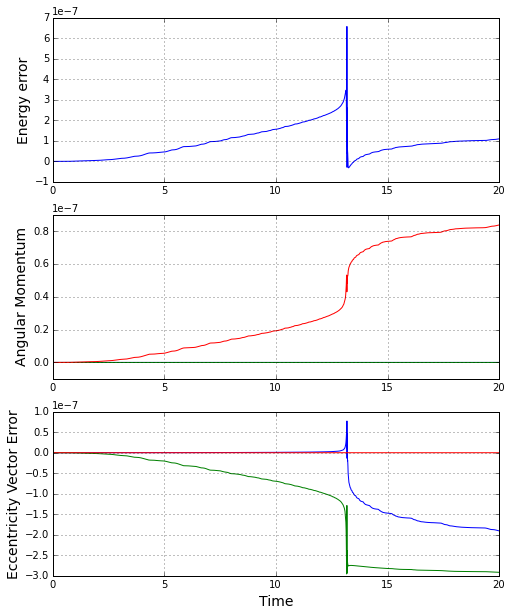
The radial equation predicts $$r_{CA} = 0.04848406$$ compared to a value of $$0.04848647$$ from the plot

Next week, I’ll be looking at the behavior of an ensemble of trajectories and will be deriving the classical scattering cross section for Rutherford scattering and examining how well the numerical experiments agree.

A couple of columns back, I strongly suggested that the definition of the scattering cross section be changed to really reflect its probabilisitic nature and that the geometric picture associated with classical scattering be eliminated. The reasons for that were expressed in the column but what I would like to add in this and subsequent columns is that I am not unsympathetic to the traditional view of the scattering cross section. In fact, I’ve had occasions to use this notion quite often in both professional and hobbyist contexts. So, in the interest of completeness, I am going to be devoting the next four columns to notions associated with scattering within the classical context.

I’ll start with the general theory of scattering from a $$1/r$$-potential. This covers both gravitational and electromagnetic forces, the two forces of classical mechanics.

The equation of motion, quite generally, is

\[ \ddot{\vec r} + \frac{\alpha \vec r}{r^3} = 0 \; .\]

where the sign of $$\alpha$$ determines whether the potential is attractive ($$\alpha > 0$$) or repulsive ($$\alpha < 0$$). Gravitational interactions are always attractive and $$\alpha$$ is usually denoted $$\mu$$ but, for generality, we’ll stick with $$\alpha$$. Now this coupled set of ordinary differential equations is readily solved numerically on just about any computer but the generation of lots of numbers doesn’t help the analysis. A better approach is to interrogate the equations of motion for conserved quantities (click here for the same approach within the context of the Maxwell equations).

Before beginning, it is useful to remind ourselves of some basic identities from many-variable calculus. The first is

\[ \frac{d}{dt} r = \frac{d}{dt} \sqrt{ x^2 + y^2 + z^2 } = \frac{1}{2 \sqrt{ x^2 + y^2 + z^2}} \frac{d}{dt} \left( x^2 + y^2 + z^2 \right) \\ = \frac{ x \dot x + y \dot y + z \dot z}{\sqrt{x^2 + y^2 + z^2}} = \frac{ \vec r \cdot \dot{\vec r} }{r} \equiv \frac{\vec r \cdot \vec v}{r} \; .\]

The second one, which follows directly from the first, is

\[ \frac{d}{dt} \left( \frac{1}{r} \right) = -\frac{ \dot {\vec r} \cdot \vec r}{r^3} \; .\]

Now, the first conserved quantity results from dotting the equation of motion with $$\vec v = \dot {\vec r}$$ to get

\[ \ddot {\vec r} \cdot \vec v + \frac{\alpha \vec r \cdot \vec v }{r^3} \; \]

The first term can be written as a total time derivative since

\[ \frac{d}{dt} \left(\frac{1}{2} \dot {\vec r} \cdot \dot {\vec r} \right) = \dot {\vec r} \cdot \ddot {\vec r} \; .\]

The second term is also a total time derivative as seen from the identities listed above. And so we get our first conserved quantity

\[ E = \frac{1}{2} \dot {\vec r} \cdot \dot {\vec r} – \frac{\alpha}{r} \equiv \frac{1}{2} \vec v \cdot \vec v – \frac{\alpha}{r} \; ,\]

which is the energy of the system.

The next conserved quantity is derived by crossing the equation of motion from the left by $$\vec r$$

\[ \vec r \times \ddot{\vec r} + \frac{\alpha \vec r \times \vec r }{r^3} = 0 \; .\]

Because of the central nature of the force, the last term is identically zero, and the remaining term

\[ \vec r \times \ddot{\vec r} = 0 \]

can be written as a total time derivative

\[ \frac{d}{dt} \left( \vec r \times \dot {\vec r} \right) = 0 \; ,\]

resulting in the conservation of angular momentum

\[ \vec L = \vec r \times \dot {\vec r} = \vec r \times \vec v \; .\]

The final conserved quantity is obtained by crossing the equation of motion from the right by the angular momentum

\[ \ddot {\vec r} \times \vec L + \frac{\alpha \vec r \times \vec L}{r^3} = 0 \; .\]

Since the angular momentum is a conserved quantity, the first term can be rewritten as

\[ \ddot {\vec r} \times \vec L = \frac{d}{dt} \left( \dot {\vec r} \times \vec L \right) = \frac{d}{dt} \left( \vec v \times \vec L \right) \; .\]

The best way to simplify the second term is to recognize that

\[ \frac{d}{dt} \frac{\vec r}{r} = \frac{\vec v}{r} – \frac{\vec r(\vec v \cdot \vec r)}{r^3} = \frac{\vec v r^2 – \vec r(\vec v \cdot \vec r)}{r^3} = -\frac{[\vec r \times (\vec r \times \vec v)]}{r^3} = – \frac{\vec r \times \vec L}{r^3} \; ,\]

where the second-to-last step results from the BAC-CAB rule and the last step is the definition of the angular momentum.

After these manipulations are completed, the resulting total time derivative is

\[ \frac{d}{dt}\left( \vec v \times \vec L – \frac{\alpha \vec r}{r} \right) = 0 \; ,\]

from which we see the conserved quantity

\[ \vec v \times \vec L – \frac{\alpha \vec r}{r} = \vec A \; .\]

This latter vector is known as the Laplace-Runge-Lenz vector.

With all these conserved quantities in place, it is relatively easy to predict certain aspects of the scattering trajectories without solving the equations directly. First, the conservation of angular momentum requires the motion to take place in the plane. As a result, plane-polar coordinates can be used to describe the motion. Since the Laplace-Runge-Lenz vector is conserved and is in the plane perpendicular to the angular momentum, it makes an excellent axis against which to measure the movement of the polar angle $$\nu$$.

\[ \vec A \cdot \vec r = A r \cos \nu \]

The variation of the radius in the plane can then be expressed as a function of $$\nu$$ as follows. Expand the dot product between $$\vec A$$ and $$\vec r$$

\[ \vec A \cdot \vec r = \left( \vec v \times \vec L – \frac{\alpha \vec r}{r} \right) \cdot \vec r = (\vec v \times \vec L) \cdot \vec r – \alpha r \; .\]

Next note, because of the cycle property of the triple-scalar product, that

\[ (\vec v \times \vec L) \cdot \vec r = (\vec r \times \vec v) \cdot \vec L = L^2 \; \]

Equating the two expressions gives

\[ A r \cos \nu = L^2 -\alpha r \; , \]

which can be readily solved to give

\[ r = \frac{L^2 / \alpha}{1 + A/\alpha \cos \nu} \;.\]

Now the interpretation of this equation requires a modest amount of care. If $$\alpha > 0$$, then the above form can immediately be recognized as a conic section with

\[ r = \frac{p}{1+e \cos \nu} \; \; \alpha > 0 ;, \]

where the semi-latus rectum $$p = L^2/\alpha$$ and the eccentricity $$e = A/\alpha$$.

If $$\alpha < 0$$, then we need to multiply the numerator and denominator by $$-1$$ to get \[ r = \frac{L^2 / |\alpha|}{A/|\alpha| \cos \nu – 1} \; , \] from which we get \[ r = \frac{p}{e \cos \nu – 1} \; ,\] where $$p = L^2/|\alpha|$$ and $$e = A/|\alpha|$$. Next week we will analyze individual scattering orbits using these conic equations and the conserved quantities.