Monthly Archive: August 2016

Starting with this installment, the focus shifts from the collective phenomenon of waves in cold plasma to the analysis of single particle motion of a charged particle under the influence of given maagnetic and electric fields. In this column, the motion in a fixed magnetic field will be analyzed. This is the most basic type of motion for plasmas and is almost always treated in the early chapters of plasma textbooks. Oddly enough, it is almost always presented in a cumbersome fashion and the cited ‘exact analytic’ solutions are usually incomplete or inaccurate. The major reason for this situation seems to be the fact that the analytic solutions are of little use in plasma physics. Nonetheless, from a pedagogical point-of-view this disconnect is a problem that should be addressed. This column is devoted to just such an aim.

The starting point is the Lorentz force law from which we obtain the equation of motion

\[ m \frac{d}{dt} \vec v = q \left( \vec E + \vec v \times \vec B \right) \; ,\]

subject to the initial conditions $$\vec r(t=0) \equiv \vec r_0$$ and $$\vec v(t=0) \equiv \vec v_0$$.

The textbook first case assumes that $$\vec E = 0$$, $$\vec B = B \hat z$$, and that the initial conditions are non-zero only in the $$x-y$$ plane. Plugging all these assumptions in yields the two equations of motion
\[ {\dot v}_x = \omega_g v_y \]

and

\[ {\dot v}_y = – \omega_g v_x \; ,\]

where the gyrofrequency is defined as

\[ \omega_g = \frac{q B}{m} \; .\]

Most textbook then try to solve these equations in rather clumsy fashion or they pass over the solution and cite analytic solutions that are incomplete or inaccurate. These will be discussed in detail below.

A much better way to solve these equations is to actually employ the standard mathematical way of solving coupled initial value problems using the fundamental matrix. The technique starts with a rewriting of the equations of motion in matrix form

\[ \frac{d}{dt} \left[ \begin{array}{c} v_x \\ v_y \end{array} \right] = \omega_g \left[ \begin{array}{cc} 0 & 1 \\ -1 & 0 \end{array} \right] \left[ \begin{array}{c} v_x \\ v_y \end{array} \right] \; .\]

The formal solution is given by
\[ \left[ \begin{array}{c} v_x \\ v_y \end{array} \right] (t) = e^{\omega_g A t} \left[ \begin{array}{c} v_{x0} \\ v_{y0} \end{array} \right] \; , \]

with the matrix

\[ A = \left[ \begin{array}{cc} 0 & 1 \\ -1 & 0 \end{array} \right] \; .\]

The matrix exponetial term is easily computed once realizes that $$A$$ squares to

\[ A^2 = \left[ \begin{array}{cc} -1 & 0 \\ 0 & -1 \end{array} \right] \; , \]

which is proportional to the unit matrix.

This is convenient since the power series form of the matrix exponential separates into two terms, each of which converges to a trigonometric function

\[ e^{\omega_g A t} = \cos (\omega_g t) 1 + \sin (\omega_g t) A \; ,\]

where $$1$$ is the $$2 \times 2$$ unit matrix.

Expansion of the fundamental matrix in terms of components results in

\[ e^{\omega_g A t} = \left[ \begin{array}{cc} \cos(\omega_g t) & \sin(\omega_g t) \\ -\sin(\omega_g t) & \cos(\omega_g t) \end{array} \right] \; .\]

Solutions to the initial value problem, in terms of initial conditions, are

\[ v_x(t) = v_{x0} \cos(\omega_g t) + v_{y0} \sin(\omega_g t) \]

and

\[ v_y(t) = -v_{x0} \sin(\omega_g t) + v_{y0} \cos(\omega_g t) \; .\]

To get the particle trajectories, one must then integrate these expressions with respect to time. There are two different ways of doing this and the choice between them is governed mostly by taste.

The first way is to perform a definite integration of both sides between $$t_0$$ (taken, for convenience, to be zero) and current time $$t$$:

\[ \int_{0}^{t} d x = \int_{0}^{t} \; dt’ \; \left( v_{x0} \cos(\omega_g t’) + v_{y0} \sin(\omega_g t’) \right) \; .\]

Explicitly computing the integrals gives

\[ x(t) – x_0 = \left. \frac{v_{x0}}{\omega_g} \sin(\omega_g t’) \right|_{0}^{t} – \left. \frac{v_{y0}}{\omega_g} \cos(\omega_g t’) \right|_{0}{t} \; ,\]

which simplifies to

\[ x(t) = x_0 + \frac{v_{y0}}{\omega_g} + \frac{v_{x0}}{\omega_g} \sin(\omega_g t) – \frac{v_{y0}}{\omega_g} \cos(\omega_g t) \; .\]

In the second method, the integrals are treated as indefinite and a single constant of integration results, giving

\[ x(t) – A = \frac{v_{x0}}{\omega_g} \sin(\omega_g t) – \frac{v_{y0}}{\omega_g} \cos(\omega_g t) \; .\]

The value of

\[ A = x_0 + \frac{v_{y0}}{\omega_g} \]

is then obtained from the initial conditions, resulting in exactly the same result.

For completeness, the result for the motion in the $$y$$ direction is

\[ y(t) = y_0 – \frac{v_{x0}}{\omega_g} + \frac{v_{x0}}{\omega_g} \cos(\omega_g t) + \frac{v_{y0}}{\omega_g} \sin(\omega_g t) \]

Interestingly, of the various textbooks examined in the field, none solve for the particle motion in the way above nor do they cite a functional form for the particle motion so derived. The most common way of tackling the equation of motion is exemplified by the treatment in Baumjohann and Treumann. They differentiate the equations once to decouple them thus arriving at

\[ {\ddot v}_x = -\omega_g^2 v_x \]

and

\[ {\ddot v}_y = -\omega_g^2 v_y \; .\]

This form has a two-fold disadvantage. First, the gyrofrequency $$\omega_g$$ appears squared here, thus losing all notion that particles of different signs in charge gyrate in different directions. Second, the second-order nature of these equations implies that there needs to be two constants of integration for the velocity evolution and a corresponding additional two for the particle motion, when, in fact, Newton’s laws require only four constants total. They fumble at with tis a bit in switching back and forth between the gyrofrequency having a sign and being the absolute value. In addition, they cite the solution to the particle equations as

\[ x – x_0 = r_g \sin( \omega_g t ) \]

and

\[ y – y_0 = r_g \cos( \omega_g t ) \; ,\]

with

\[ r_g \frac{v_{\perp}}{|\omega_g|} \; .\]

Chen tackles the equations similarly, deriving the velocity double-dot form before presenting the solution for the particle motion of

\[ x – x_0 = -i e^{-\omega_g t} \]

and

\[ y – y_0 = \pm e^{-\omega_g t} \; ,\]

which become, upon taking the real part,

\[ x – x_0 = r_g \sin( \omega_g t ) \]

and

\[ y – y_0 = \pm r_g \cos( \omega_g t ) \; .\]

He make no mention as to when to use the two different signs.

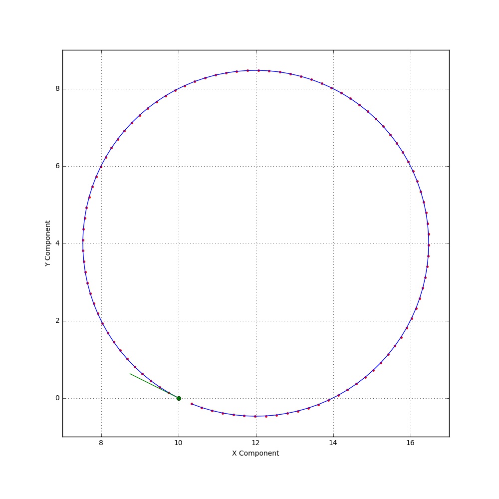
In order to see that the solution is derived in this column is correct, a numerical simulation of the equations of motion was implemented in Python, using the IPython/Jupyter framework with numpy and scipy extensions. The figures below show the initial conditions – initial position (green dot) and initial velocity (green line) – and the resulting motion from the numerical integration (blue line) with the analytic solution (red and black dot for positive and negative charge).

Positive Charge

Negative Charge

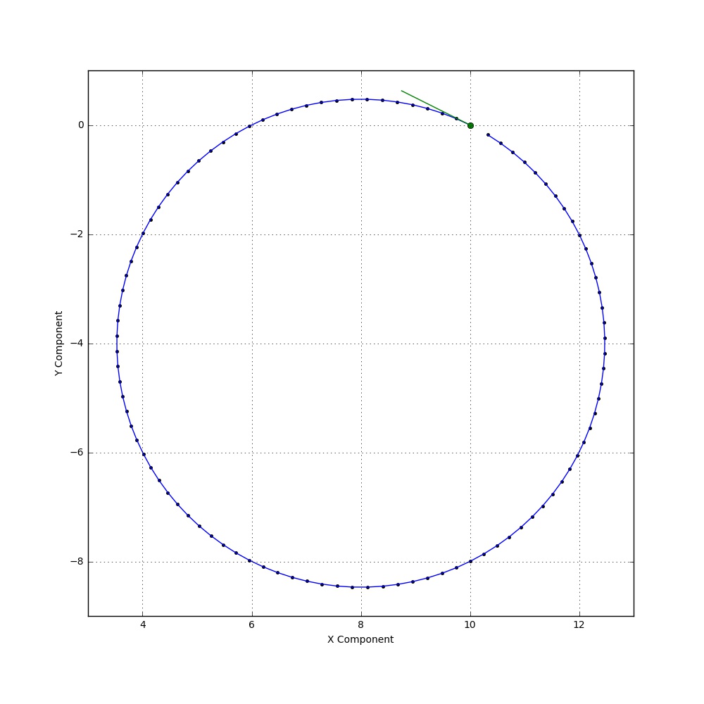
The agreement is excellent, showing the necessity of the ‘extra’ terms here derived. Also note that the sense of rotation is opposite for the negative charge compared to the positive one.