
Plasma Oscillations
This month’s installment focuses on that aspect of plasma dynamics that is strongly analogous with mechanical vibration: plasma oscillations. Plasma oscillations were first predicted by Paul Langmuir in the 1920s and later observed in vacuum tubes of the day.
These oscillations manifest themselves as cooperative movements in a plasma’s charge distribution that behave sinusoidalally. The harmonic nature of these deviations from perfect neutrality is basically due to an electrostatic restoring force that, for small amplitudes around equilibrium, is well approximated as quadratic. Thus the electrostatic restoring force gives rise to a harmonic potential. The analog with mechanical oscillations is completed with the identification of the electron and ion centers-of-mass velocities with the macroscopic kinetic energy of the mass on the spring. Plasma oscillations provide strong support for the basic assumptions of electromagnetic theory and a nice example of how mechanics and electrodynamics meet in a physically relevant situation.
The aim here is to derive the formulae for the plasma oscillations for two related cases and then to interpret the results in terms of mechanical vibration with the familiar spring mass system.
Imagine that there is a slab of plasma of length $$\ell_0$$, with cross-sectional area $$A$$ and an initial number density of ions and electrons of $$n_0$$. Since the condition of quasi-neutrality is in effect, there is no net electric field in any part of the plasma. Now imagine that due to an outside agency, all of the electrons are displaced by the very small amount of $$\Delta x$$ to the left, leaving a net positive charge on the right and net negative charge on the left, with the thickness of these two ‘non-neutral’ regions is $$\Delta x$$.
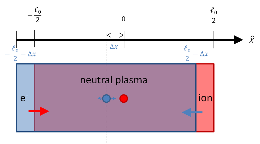
How does the plasma respond to this out of equilibrium condition? The first approximation one can make is that the electrons are free to move but the ions are fixed in space. This corresponds to the physical approximation that the ions have an infinite mass – an approximation that is well supported by the ~2000 – 1 ratio between the mass of a proton and that of an electron.
The electrons will feel a strong restoring force (red arrow) and they will move accordingly. Since the ions are fixed, they will feel an equal but opposite restoring force (blue arrow) but they will not be able to respond.
The electric field that the electrons and ions will feel, which is most easily obtained from Gauss’s law, is non-zero between the strips of positive and negative charge in an exactly analogous fashion as to the textbook problem on parallel plate capacitors. The density of ions in the red region is $$n_0$$ and the volume is $$A \Delta x$$. Since $$\Delta x$$ is small compared to the other dimensions, the electric field is closely approximated as being entirely in the $$x$$-direction and the total flux through a Gaussian surface whose boundaries coincide with the ion region is due strictly to the left and right faces. The right face flux is exactly zero since the flux from the electrons exactly cancels the flux from the ions. The left face flux, which is equal to the total flux, is then
\[ \Phi_E = E A \; , \]
which is proportional to the total charge enclosed
\[ \Phi_E = \frac{e n_0 A \Delta x}{\epsilon_0} \; .\]
Equating gives
\[ E= \frac{e n_0 }{\epsilon_0 } \Delta x \; ,\]
which is the usual result for the field between a parallel plate capacitor ($$n_0 \Delta x$$ is the surface charge density).
As the electrons were all displaced uniformly and are experiencing a uniform force, they will move together as a unit, that is to say cooperatively. The mass of the unit is simply the mass density $$m_e n_0$$ times the volume consumed $$V = A \ell_0$$. The center of mass of the slab is at $$\ell/2- \Delta x$$ with the corresponding acceleration $$\Delta {\ddot x}$$. The force on the slab is
\[ F = q_{tot} E = -e n_0 V \frac{e n_0}{ \epsilon_0} \Delta x\]
and the equation of motion of the entire slab is given by:
\[ m_e n_0 V \frac{d^2}{dt^2} \Delta x = -e n_0 V \frac{e n_0} {\epsilon_0} \Delta x \; .\]
Dividing out the common factors gives
\[ \frac{d^2}{dt^2} \Delta x = -\frac{e^2 n_0}{m_e \epsilon_0} \Delta x \; .\]
From this equation we would conclude that, for small displacements, the electron slab would oscillate at the angular frequency
\[ \omega_{pe} = \sqrt{ \frac{e^2 n_0}{m_e \epsilon_0} } \; , \]
which is called the electron plasma frequency (note it is really an angular frequency).
Relaxing the assumption that the ions don’t move makes the analysis somewhat more complicated but only changes the result in a small but crucial way. The location of both electron and ion centers-of-mass now matter and must be tracked separately. The picture of their motion is now
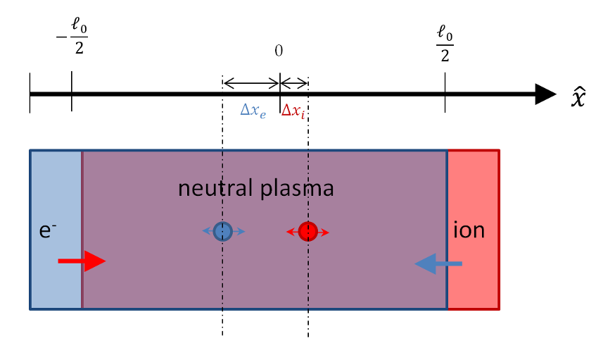
Since both species are free to move, the thickness of the exposed electron or ion regions (red and blue) is not determined solely by the movement of their respective centers-of-mass (the ion region pictured above is much larger than $$\Delta x_i$$) . The total thickness of the exposed regions depends on the relative motion between both centers-of-mass
\[ t = \Delta x_i – \Delta x_e \; .\]
An initial analysis may suggest that there are 8 separate cases: positive or negative variations for each species (2×2) as well as whether the ions are more displaced versus the electrons. In fact, there are only two cases based on whether $$t$$ is positive (ion strip is on the right) or whether $$t$$ is negative (ion strip is to the left). The following table shows the 8 variations for $$\ell = 1$$.
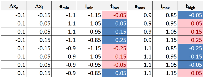
The parameters with the ‘min’ designate the leftmost extent of the electron slab ($$e_{min}$$) and the ion slab ($$i_{min}$$). The parameter $$t_{low} = i_{min} – e_{min}$$. A negative value, such as in case 1, means that the ion slab has shifted more to the left than the electrons and that the exposed ion region (red) is now on the left while the exposed electron region (blue) is now on the right. A positive value of $$t_{low}$$ means the converse. The corresponding parameters at the rightmost side are defined in an analogous fashion. The color coding assists in visualizing which species is in which location. Note that the entire table can be summarized by $$\Delta x_i – \Delta x_e$$, whose magnitude and sign match $$t_{low}$$ and $$t_{high}$$. Also note that the displacements in the table are purely geometric and that the actual dynamic displacements would not shift the total center-of-mass since the only forces in the problem are internal.
The electric field in between the two uncovered charge regions can also be obtained by Gauss’s law, but it is instructive to use the expression for the electric field due to a sheet of charge that and superposition. The electric field due to the ions will have a magnitude of
\[ E_i = \frac{e n_0}{2 \epsilon_0} \left(\Delta x_i – \Delta x_e \right) \]
using the standard result from elementary E&M.
Likewise the electric field due to the electrons will also have the same magnitude $$E_e = E_i$$. Their directions will be the same in the region between them (the neutral plasma) and opposite outside, so that a non-zero field with magnitude $$2 E_i$$ will result only in the middle region. The direction of the field depends on which one is on the right versus the left but it doesn’t matter for the sake of the dynamical analysis.
The equation of motion for each slab is then given by
\[ m_i \frac{d^2}{dt^2} \Delta x_i = -\frac{e^2 n_0}{\epsilon_0} \left(\Delta x_i – \Delta x_e\right) \]
and
\[ m_e \frac{d^2}{dt^2} \Delta x_e = \frac{e^2 n_0}{\epsilon_0} \left(\Delta x_i – \Delta x_e\right) \; . \]
Combining these two equations gives
\[ \frac{d^2}{dt^2} \left( \Delta x_i – \Delta x_e \right) = -\frac{e^2 n_0}{\epsilon_0}\left(\frac{1}{m_e} + \frac{1}{m_i} \right) \left(\Delta x_i – \Delta x_e\right) \]
from which we conclude that the frequency is now
\[ \omega_p^2 = \frac{e^2 n_0}{\epsilon_0}\left(\frac{1}{m_e} + \frac{1}{m_i} \right) = \frac{e^2 n_0}{\epsilon_0 m_e} + \frac{e^2 n_0}{\epsilon_0 m_i} \equiv \omega_{pe}^2 + \omega_{pi}^2 \; .\]
The above analysis has a direct analog in a mechanical system of two unequal masses $$m_1$$ and $$M_2$$ connected by a spring of spring constant $$k$$ and equilibrium length $$\ell_0$$.
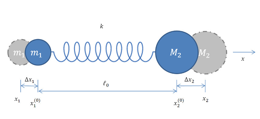
Defining the deviations of each mass from the equilibrium positions as
\[ \Delta x_1 = x_1 – x_1^{(0)} \]
and
\[ \Delta x_2 = x_2 – x_2^{(0)} \]
the distance between them takes the form
\[ x_2 – x_1 = x_2^{(0)} + \Delta x_2 – x_1^{(0)} – \Delta x_1 \equiv \ell \; .\]
Combining these two definitions gives
\[ x_2 – x_1 = \Delta x_2 – \Delta x_1 + \ell_0 \equiv \delta \ell + \ell_0 \]
from which the potential follows as
\[ V = \frac{1}{2} k (\ell – \ell_0)^2 = \frac{1}{2} k (\Delta x_2 – \Delta x_1)^2 \; .\]
The Lagrangian takes the form
\[ L = \frac{1}{2} m_1 \Delta \dot x_1^2 + \frac{1}{2} M_2 \Delta \dot x_2^2 – \frac{1}{2} k (\Delta x_2 – \Delta x_1)^2 \; , \]
with the equations of motion becoming
\[ \frac{d}{dt} \frac{\partial L}{\partial \dot x_1} – \frac{\partial L}{\partial x_1} = m_1 \Delta \ddot x_1 + k(\Delta x_2 – \Delta x_1 ) = 0 \]
and
\[ \frac{d}{dt} \frac{\partial L}{\partial \dot x_2} – \frac{\partial L}{\partial x_2} = M_2 \Delta \ddot x_2 – k(\Delta x_2 – \Delta x_1 ) = 0 \]
These equations combine nicely into one expression for the dynamics of the change in the separation between the two masses
\[ \delta \ddot \ell = -\left( \frac{k}{m_1} + \frac{k}{M_2} \right) \delta \ell \; , \]
which immediately tells us that the frequency of the oscillations is given by
\[ \omega^2 = k \left(\frac{1}{m_1} + \frac{1}{M_2} \right) = \omega_1^2 + \omega_2^2 \; .\]
In the limit as $$ M_2 \rightarrow \infty $$, the equation of motion simplifies to
\[ \delta \ddot \ell + \frac{k}{m_1} \delta \ell = 0 \; ,\]
with frequency of
\[ \omega^2 = \frac{k}{m_1} = \omega_1^2 \; .\]
Thus there is a perfect analogy between the two pictures and the cooperative motion of the electrons and ions within the plasma can be interpreted in strictly mechanical terms.