
Dipole Field Lines and the Earth
As pointed out in an article entitled Field Pattern of a magnetic dipole (Am. J. Phys. 68 (6), June 2000), J. P. Mc Tavish, notes that while it is common to see a treatment of the magnetic dipole in essentially every electromagnetic text, it is all too rare to find a discussion on how to draw the field lines. While Mc Tavish’s article is successful in remedying that shortfall, it omits any connection with specific physical situations, in particular with the most important dipole magnet to the human race: the one on which we live – the Earth.
Alternatively, in the space physics community it is all too common to see the physical connection to the Earth’s dipole field and corresponding field lines but the basic physics associated with deriving these equations from Maxwell’s equations to the dipole is usually missing. And those that do (e.g. the very instructive lecture by Ling-Hsaio Lyu) often cut some vital parts.
It is the intention of this post to create a single narrative that starts from first principles and ends with the standard space physics expression for the Earth’s dipole field in terms of the standard L-shells. The bulk of the initial part of this post is based on the treatment of the dipole in Foundations of Electromagnetic Theory by Reitz, Milford, and Christy.
The starting point is the monopole law $$\vec \nabla \cdot \vec B = 0$$, which asserts that the magnetic field is purely solenoidal, and, as a result, can be written in terms of the vector potential $$\vec A$$ as
\[ \vec B = \vec \nabla \times \vec A \; . \]
Since we want the description of an isolated magnetic dipole field, two immediate conditions can be place on Maxwell’s equations: $$\partial_t \vec B = 0$$ and $$\rho = 0$$. The only non-trivial Maxwell equation is now the Ampere-Maxwell law, that states (subject to the earlier conditions)
\[ \vec \nabla \times \vec B = \mu_0 \vec J \; . \]
Substituting in the vector potential yields
\[ \vec \nabla \times (\vec \nabla \vec A) = \mu_0 \vec J \; .\]
Expanding the double-curl with the standard vector identity leads to
\[ \vec \nabla (\vec \nabla \cdot \vec A) – \nabla^2 \vec A = \mu_0 \vec J \; , \]
which can be further reduced by picking the Lorentz gauge, which sets $$ \vec \nabla \cdot \vec A = 0 $$. This choice leads to the final equation
\[ \nabla^2 \vec A = -\mu_0 \vec J \; ,\]
which asserts that each component of the vector potential obeys a Poisson equation with the source being $$\mu_0 \vec J$$. The solution of these three equations follows by analogy with electrostatics and the result is
\[ \vec A(\vec r) = \frac{\mu_0}{4 \pi} \int d^3 r’ \frac{\vec J(\vec r \,’)}{|\vec r – \vec r \,’|} \; . \]
Now for most dipoles (microscopically contained in matter or the Earth), the field is generally distant from the source point ($$|\vec r| >> |\vec r \,’| $$). This relation suggests a multipole expansion of the Green’s function
\[ |\vec r – \vec r \,’|^{-1} = (r^2 + r’^2 – 2 \vec r \cdot \vec r \,’)^{-1/2} \; . \]
The dipole is the first-order piece of such an expansion, so we can approximate the Green’s function as
\[ |\vec r – \vec r \,’|^{-1} = \frac{1}{r} \left[ 1 + \frac{\vec r \cdot \vec r \,’}{r^2} \right] \; . \]
One additional approximation is needed; assume that the currents creating the dipole are bound and an be idealized as flowing through a “thin wire” (effectively a Dirac delta function is used to localize the current into a circuit whose characteristic sizes are small compared to all other lengths being considered). In this case, the volume integral becomes a closed line integral. Under this modest approximation:
\[ \vec A(\vec r) = \frac{\mu_0 I}{4 \pi} \left\{ \frac{1}{r} \oint d \vec r \,’ + \frac{1}{r^3} \oint d \vec r \,’ \vec r \cdot \vec r \,’ \right \} \; . \]
The first integral vanishes since the line integral forms a close loop. The second integral, refered hereafter as the dipole integral, requires some ingenuity, all of which is supplied by Rietz, Milford, and Christy (Sec. 8.7). The first step in dealing with the dipole integral comes from noting (using back-cab) that
\[ (\vec r \,’ \times d \vec r \,’) \times \vec r = – \vec r \times (\vec r \,’ \times d \vec r \,’) = \\ – [ \vec r \,’ (\vec r \cdot d \vec r \,’) – d \vec r \,’ (\vec r \cdot \vec r \,’) ] = d\vec r \,’ (\vec r \cdot \vec r \,’) – \vec r \,’ (\vec r \cdot d \vec r \,’) \; .\]
To eliminate the first term employ the identity
\[ d[ \vec r \,’ (\vec r \cdot \vec r \,’) ] = d \vec r \,’ (\vec r \cdot \vec r \,’) + \vec r \,’ (\vec r \cdot d \vec r \,’) \; \]
that results from a change in $$\vec r \,’$$ keeping $$\vec r$$ fixed.
Now add the two previous expressions together to get
\[ (\vec r \,’ \times d \vec r \,’) \times \vec r + d[ \vec r \,’ (\vec r \,’ \cdot \vec r) ] = 2 d \vec r \,’ (\vec r \cdot \vec r \,’) \; , \]
which, when divided by 2 and substituted into the dipole integral gives
\[ \vec A (\vec r) = \frac{\mu_0 I}{4 \pi r^3} \frac{1}{2} \oint \left\{ (\vec r \,’ \times d \vec r \,’) \times \vec r + d[\vec r \,’ (\vec r \,’ \cdot \vec r) ] \right \} \; . \]
The second terms is identically zero, since it an exact differential. The first terms can be suggestively rearranged to give
\[ \vec A(\vec r) = \frac{\mu_0}{4 \pi} \left\{ \oint \frac{I}{2} (\vec r \,’ \times d \vec r \,’) \right\} \times \frac{\vec r}{r^3} \equiv \frac{\mu_0}{4 \pi} \vec m \times \frac{\vec r}{r^3} \; , \]
where $$\vec m$$ is defined as the magnetic dipole (or magnetic dipole moment).
Before computing $$\vec B$$, let’s take a moment to think about the definition of $$\vec m$$. Consider an arbitrary current-carrying loop
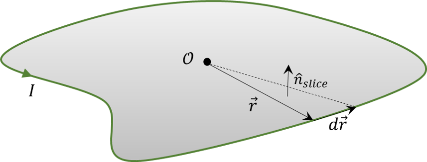
where the origin is chosen near the loop. The differential vector $$\vec r \,’ \times d \vec r \,’$$ is normal to a small slice of area. Summing each piece in the integral results in an expression that roughly says
\[ \vec m = \frac{\mu_0}{4 \pi} I \left( \frac{1}{2} \oint \vec r \,’ \times d \vec r \,’ \right) = \frac{\mu_0}{4 \pi} I \, Area \, \hat n \; , \]
but the area has each slice weighted differently, based on how far from the origin it excursion takes it. As a side note, Griffiths calls this the directed area and obtains it from the Stoke’s theorem by an ingenious substitution for the vector field in question (seems like some degree of cleverness is required no matter how one does this analysis).
The next step is to calculate the magnetic field. Taking the curl gives
\[ \vec B (\vec r) = \vec \nabla \times \vec A(\vec r) = \vec \nabla \times \left( \frac{\mu_0}{4 \pi} \vec m \times \frac{\vec r}{r^3} \right) \; .\]
To expand the right-hand side, use index notation (starting with $$\vec A \times \vec B = \epsilon_{ijk} A_j B_k$$)
\[ \vec \nabla \times \left( \frac{\mu_0}{4 \pi} \vec m \times \frac{\vec r}{r^3} \right) = \frac{\mu_0}{4 \pi} \epsilon_{ijk} \epsilon_{k \ell m} \partial_j m_{\ell} \frac{r_m}{r^3} \; . \]
Cyclically permute the indices on $$\epsilon_{k \ell m}$$ to get
\[ \frac{\mu_0}{4 \pi} \epsilon_{ijk} \epsilon_{k \ell m} \partial_j m_{\ell} \frac{r_m}{r^3} = \frac{\mu_0}{4 \pi} \epsilon_{ijk} \epsilon_{\ell m k} \partial_j m_{\ell} \frac{r_m}{r^3} \; . \]
Now use the standard identity
\[ \epsilon_{ijk} \epsilon_{\ell mk} = \delta_{i \ell} \delta _{jm} – \delta_{im} \delta_{j \ell} \; .\]
to get
\[ \frac{\mu_0}{4 \pi} \epsilon_{ijk} \epsilon_{\ell m k} \partial_j m_{\ell} \frac{r_m}{r^3} = \frac{\mu_0}{4 \pi} \left( \delta_{i \ell} \delta _{jm} – \delta_{im} \delta_{j \ell} \right) \partial_j m_{\ell} \frac{r_m}{r^3} \; .\]
Expanding gives
\[ \frac{\mu_0}{4 \pi} \epsilon_{ijk} \epsilon_{\ell m k} \partial_j m_{\ell} \frac{r_m}{r^3} = \frac{\mu_0}{4 \pi} \left[ m_i \partial_j \left( \frac{r_j}{r^3} \right) – m_j \partial_j \left( \frac{r_i}{r^3} \right) \right ] \; .\]
Now focus on the term inside the square brackets. Operating with the derivatives gives
\[ m_i \partial_j \left( \frac{r_j}{r^3} \right) – m_j \partial_j \left( \frac{r_i}{r^3} \right) = m_i \frac{3}{r^3} – 3 m_i \frac{r_j r_j}{r^5} – m_j \frac{\delta_{ij}}{r^3} + m_j \frac{3 r_i r_j}{r^5} \; . \]
The first two terms vanish and the second two, when put into vector notation, give for the magnetic field
\[ \vec B(\vec r) = \frac{\mu_0}{4 \pi} \left[ -\frac{\vec m}{r^3} + 3 \frac{(\vec m \cdot \vec r) \vec r}{r^5} \right] \; .\]
With this form in hand, it is possible to calculate the field lines. There are two ways to do this: in Cartesian coordinates and in spherical coordinates. Either is fine, but spherical coordinates affords some advantages in space physics and will be pursued here.
That said, both cases benefit from exploiting axial symmetry and, without loss of generality, the analysis will be confined to the $$x-z$$ plane.
The geometry is shown below.
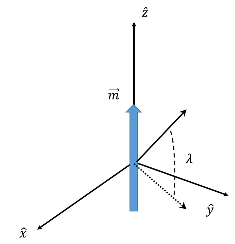
To put the coordinate-free expression into polar coordinates we need to express the vectors in terms of the basis $$\left\{ \hat r, \hat \lambda, \hat \phi \right\}$$ (although we are supressing $$\hat \phi$$ by exploiting the azimuthal symmetry).
Starting with the position vector
\[ \vec r = r \cos \lambda \, \hat x + r \sin \lambda \, \hat z \; \]
gives
\[ \hat r = \frac{\partial \vec r}{\partial r} = \cos \lambda \, \hat x + \sin \lambda \, \hat z \; , \]
and
\[ \hat \lambda = \frac{\partial \vec r}{\partial \lambda} / \left| \frac{\partial \vec r}{\partial \lambda} \right| = – \sin \lambda \, \hat x + \cos \lambda \, \hat z \; . \]
Inverting these relations gives
\[ \hat z = \sin \lambda \, \hat r + \cos \lambda \, \hat \lambda \; .\]
Since $$\vec m = m \hat z$$, the magnetic field becomes
\[ \vec B = \frac{m \mu_0}{4 \pi r^3} \left[ 3 \frac{ (\vec m \cdot \vec r) \vec r }{r^2} – \vec m \right] = \frac{m \mu_0}{4 \pi r^3} \left[ 2 \sin \lambda \, \hat r – \cos \lambda \, \hat \lambda \right] \; , \]
giving
\[ B_r = \frac{D}{r^3} 2 \sin \lambda \; \]
and
\[ B_{\lambda} = \, -\frac{D}{r^3} \cos \lambda \; , \]
where $$D = m \mu_0 /4 \pi$$.
The final piece is to get an equation of the form $$r = r(\lambda)$$ so that we can get the field lines. From Section 3.2 of Introduction to Vector Analysis by David and Snider, the tangent field to the field lines is given by $$\vec T = \beta \vec B$$, where $$\beta$$ is an arbitrary, and ultimately, inconsequential, constant. In coordinates, this expression leads to the vector equation
\[ \vec T = \frac{d r}{d s} \hat r + r \frac{d \lambda}{d s} \hat \lambda = B_r \hat r + B_{\lambda} \hat \lambda \; , \]
which gives
\[ \frac{dr}{B_r} = \frac{r d \lambda}{B_{\lambda}} \; . \]
This equation is recast as follows:
\[ \frac{dr}{r} = \frac{B_r}{B_{\lambda}} d \lambda = \, – \frac{2 \sin \lambda}{\cos \lambda} d \lambda = 2 \frac{d(\cos \lambda)}{\cos \lambda} \; . \]
The solution is readily obtained by integrating from the equation towards the pole (symmetry again)
\[ \int_{r_{eq}}^{r} \frac{dr’}{r’} = \int_{1}^{\cos \lambda} 2 \frac{ d(\cos \lambda) }{ \cos \lambda } = \int_{1}^{\cos \lambda} 2 \frac{ dx }{x} \; , \]
giving
\[ \left. \ln(r’) \right|^r_{r_{eq}} = \left. \ln( x^2 ) \right|_1^{\cos \lambda} \; , \]
which simplifies to
\[ \ln(r)- \ln(r_{eq}) = \ln(\cos^2 \lambda) – \ln(1) \; . \]
The final form is
\[ r(\lambda) = r_{eq} \cos^2 \lambda = L R_e \cos^2 \lambda \; . \]
The parameter $$L$$ labels the fieldline and different fieldlines intersect the Earth’s surface at different latitudes.
`