
Continuum Mechanics 1 – Material Derivative
This post marks the beginning of a detailed study of continuum mechanics. There are many reasons behind this study. On the physical front, the applications are numerous and important. Studies of elasticity are crucial in understanding the behavior of materials in diverse settings from man-made structures like cars, bridges, and buildings to naturally occurring applications like plate tectonics. Fluid mechanics is ubiquitous, being involved in all aspects of industrial and academic endeavors. Continuum mechanics also plays a role in such cutting-edge disciplines as plasma physics and general relativity.
Unfortunately, the study of continuum mechanics involves a number of difficulties at all levels of inquiry.
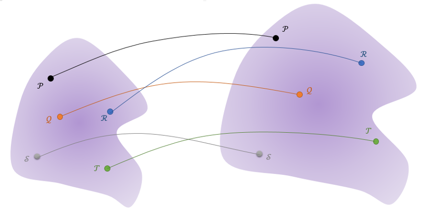
First and foremost is the philosophical difficulty associated with reconciling the atomic nature of matter with the concept of a continuous field. Consider a portion of a substance whose atomic constituents are labeled
\[ \mathcal{P}, \mathcal{Q}, \mathcal{R}, \mathcal{S}, \mathcal{T} \; .\]
We imagine that each particle moves along a trajectory parameterized by $$t$$; that there is a mapping $$\Phi$$ that flows particle $$\mathcal{P}$$ from its position at $$\vec a_{\mathcal{P}}(t_0)$$ to $$\vec a_{\mathcal{P}}(t)$$:
\[ \Phi: \vec a_{\mathcal{P}}(t_0) \rightarrow \vec a_{\mathcal{P}}(t) \; . \]
Assuming the trajectories are continuous and smooth (i.e. putting aside the possibility of stochastic or quantum motion), so that the mapping $$\Phi$$ is differentiable, there remains many questions as to how a swarm of particles can be smeared or smoothed into a continuum.
The usual prescription is to employ the notion of a material or fluid element, whose volume is large enough to fit an enormous number of particles, so that smoothing can be done by taking averages, but small enough so that there are no appreciable changes across its extent. That, this balancing act between the too small and the too large presents itself in many physical situations is one of the miracles of continuum mechanics.
There are additional considerations about any restrictions that should be placed on the continuum motion. Can the trajectories cross so long as two elements don’t occupy the same point at the same time (see the above figure). Do all the mathematical functions used in the model need to be single-valued, continuous, or differentiable?
The next set of difficulties involve a host of technical details. Three stick out in particular: distinguishing between Lagrangian and Eulerian points-of-view, the mathematical way to construct the model of how the movement of the individual material particles will be tracked, and the eternal problem of notation and the associated bookkeeping.
In the Lagrangian viewpoint, attention is fixed on a material or fluid element and follows its motion as it flows. This viewpoint is akin to sitting in a boat as it moves down a river. The surroundings change and the banks slip by as the boat follows the piece of water on which it floats. The Lagrangian viewpoint is the one in which Newton’s laws may be applied with almost the same ease as in particle mechanics. The position, velocity, and acceleration of an element surrounding $$\mathcal{P}$$ follows the well-defined trajectory
\[ \vec a_{\mathcal{P}}(t) \; .\]
In the Eulerian viewpoint, attention is fixed on the locale and the various material or fluid elements which enter and leave this region are only briefly viewed before being lost. Each airplane traveler who sits by the window over a wing and contemplates the lift generated as air rushes over it experiences the Eulerian viewpoint even if they are unaware of the finer points. The Eulerian viewpoint is most commonly used in physical analysis since measurements are made at specific points and devices like valves and pipes and the like are fixed in space $$\vec r$$.
Connection between these two viewpoints is affected through the material derivative.
The material derivative, which has many aliases (such as the total or Lagrangian derivative – Wikipedia lists 10 of them), is based on the idea of how a set of trajectories fills a space. Consider the path of two elements $$\mathcal{P}$$ and $$\mathcal{Q}$$ as they move along the red trajectory.
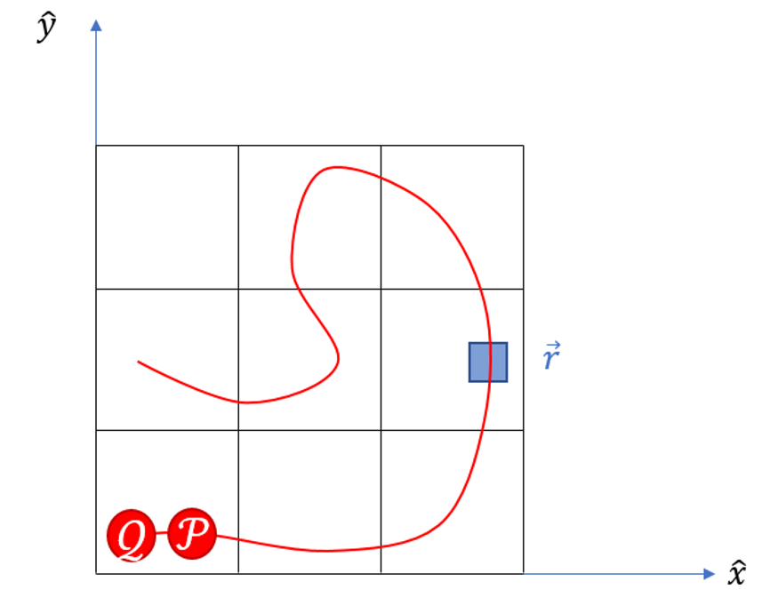
At some given time $$t_0$$ they are positioned as pictured at $$\vec a_{\mathcal{P}}$$ and $$\vec a_{\mathcal{Q}}$$. At some later time $$t_1$$, $$\mathcal{P}$$ enters the blue box at $$\vec r$$. Shortly afterwards, at $$t_2$$, $$\mathcal{Q}$$ enters the same position. By noting the time and the starting point of each of these two elements, we can determine their respective positions at all later times. Generalizing to a continuum, there exists, at least conceptually, a function
\[ \vec R(\vec a,t) \]
that spits out the position of an element that started at position $$\vec a$$ at time $$t_0$$. A moment’s reflection should convince one that a proper boundary condition on $$\vec R$$ is
\[ \vec R(\vec a,t_0) = \vec a \; ,\]
that is the mapping is the identity at the initial time.
Since no two elements are allowed to occupy the same position at the same time, the function $$\vec R$$ can be inverted, again at least conceptually, so that we have a function
\[ \vec A(\vec r,t) \; .\]
This function works in a complementary fashion, telling us which of the elements is at $$\vec r$$ (blue box) at time $$t$$. Its boundary condition at time $$t_0$$ has to be
\[ \vec A(\vec r,t_0) = \vec a \; , \]
since it has to coincide with $$\vec R$$ as an identity at the initial time ($$\vec A$$ and $$\vec R$$ are inverse mappings – if $$\vec R$$ is the identity then so must $$\vec A$$).
With this machinery in place, one can move back and forth between the trajectory (Lagrangian) and the field (Eulerian) points-of-view.
Now suppose that there are two observers, one that rides along with $$\mathcal{P}$$ and the other sitting in the blue box at $$\vec r$$, and suppose that each of them measures the temperature frequently. Obviously, they must agree on the temperature only at $$t_1$$ when $$\vec R({\vec a_{\mathcal{P}},t_1}) = \vec r$$. But will they agree on the rate of change in the temperature?
Generally, the answer is no for the following reason. If the temperature field at each point and time in the space is given by $$T(x,y,z)$$ then the observer at $$\vec r$$ will see a rate of change of
\[ dT = \left. \frac{\partial T}{\partial t} \right|_{x,y=x_{\vec r},y_{\vec r}} dt \; ,\]
since the position remains unchanged (as emphasized by the standard notation on the partial derivative – for clarity of notation, this emphasis will be dropped hereafter).
The observer co-moving with $$\mathcal{P}$$ must plug his trajectory into $$T$$ to give
\[ T\left( X(\vec a,t), Y(\vec a,t), t \right) \]
with a corresponding change given by
\[ dT = \frac{\partial T}{\partial t} dt + \frac{\partial T}{\partial x} dx + \frac{\partial T}{\partial y} dy \; .\]
The time rate of change is given by dividing both sides by $$dt$$ to give
\[ \frac{dT}{dt} = \frac{\partial T}{\partial t} + \frac{\partial T}{\partial x} \frac{dx}{dt} + \frac{\partial T}{\partial y} \frac{dy}{dt} \; ,\]
which, in vector notation, gives the usual form of the material derivative
\[ \frac{dT}{dt} = \frac{\partial T}{\partial t} + \vec v \cdot \nabla T \; .\]
The next post will explore the material derivative in a concrete example. In the following posts, the material derivative will be the primary tool for relating Newton’s laws in the Lagrangian picture to the field equations in the Eulerian picture.