
Continuum Mechanics 3 – Reynolds Transport Theorem
The last two posts thoroughly explored the material derivative, which is the primary means of moving between the Lagrangian point-of-view (follows a fluid element as it moves) and the Eulerian point-of-view (watches multiple fluid elements moving past a point in space). The next ingredient are the Reynolds and Flux transport theorems that relate determine the time rate of change of some property (typically volumetric and surface properties, respectively) as the material moves and its bounding surface evolves.
The approach in this post will be to work up from a simple example to the complete Reynolds theorem. The next post will then use the Reynolds theorem to motivate the Flux transport theorem and then generalize it as the last step. The treatment here is strongly influenced by Introduction to Vector Analysis, 4th ed. By Davis and Snider but I’ve inverted the logical ordering since the Reynolds theorem is more central to the study of fluids than the Flux transport theorem.
Consider a cubic fluid element with a corner $$\mathcal A$$ located at the point $$\vec r_{\mathcal A} = x \hat \imath + y \hat \jmath + z \hat k$$.
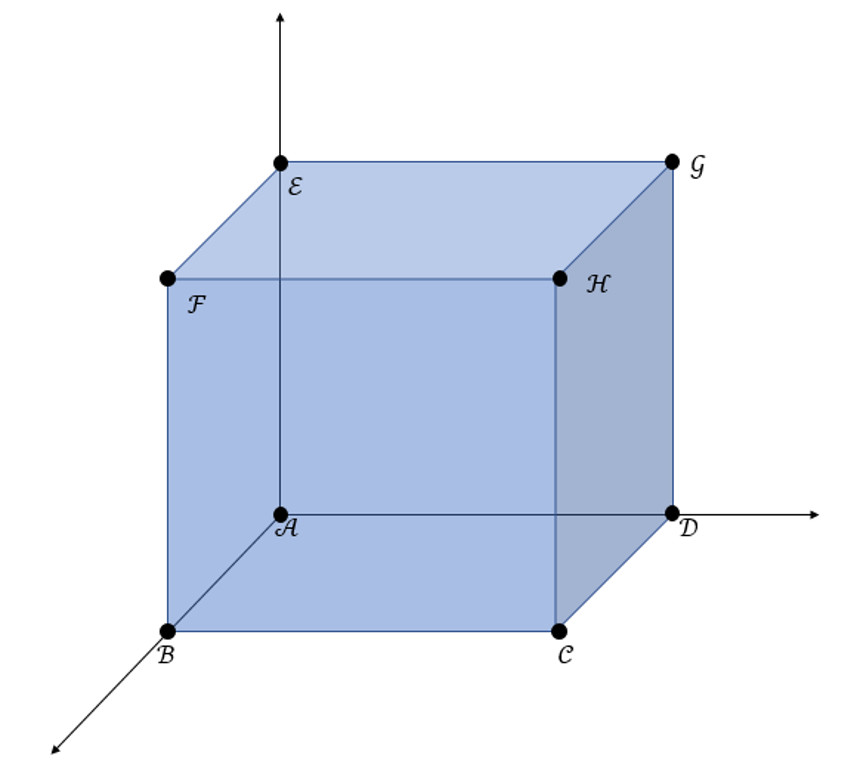
If the extent of the cube is $$\Delta x$$, $$\Delta y$$, and $$\Delta z$$ along those three dimensions, then the other points are found at
\[ \vec r_{\mathcal B} = (x+\Delta x) \hat \imath + y \hat \jmath + z \hat k \; \, \]
\[ \vec r_{\mathcal C} = (x + \Delta x) \hat \imath + (y+\Delta y) \hat \jmath + z \hat k \; \, \]
\[ \vec r_{\mathcal D} = x \hat \imath + (y+\Delta y) \hat \jmath + z \hat k \; \, \]
\[ \vec r_{\mathcal E} = x \hat \imath + y \hat \jmath + (z + \Delta z) \hat k \; \, \]
and so on.
The volume of this cube is obviously $${\mathcal V}ol = \Delta x \Delta y \Delta z$$ but it will be helpful for what follows to also see that the same results follows from the triple scalar product.
In this case, we need three vectors lying along three independent, orthogonal sides. The easiest ones to use are the sides connecting $$\mathcal A$$ to $$\mathcal B$$, $$\mathcal A$$ to $$\mathcal D$$, and $$\mathcal A$$ to $$\mathcal E$$. The corresponding vectors are:
\[ \vec r_x = \vec r_{\mathcal B} – \vec r_{\mathcal A} = \Delta x \hat \imath \; ,\]
\[ \vec r_y = \vec r_{\mathcal D} – \vec r_{\mathcal A} = \Delta y \hat \jmath \; ,\]
and
\[ \vec r_z = \vec r_{\mathcal E} – \vec r_{\mathcal A} = \Delta z \hat k \; .\]
The triple product $$\vec r_x \cdot (\vec r_y \times \vec r_z)$$ gives the volume as before.
Next consider the situation where the fluid element flows. Generically, the velocity at each point in the fluid element will be determined by the function $$\vec V(x,y,z)$$. This means that the velocity at each corner will be different and that the volume of the fluid element will change as it flows. The Reynolds transport theorem describes by how much the volume changes per unit time.
In a small amount of elapsed time, $$\Delta t$$, the corner at $$\mathcal A$$ will move to
\[ \vec r\;’_{\mathcal A} = \vec r_{\mathcal A} + \Delta t \; \vec V(x,y,z) \; . \]
Likewise, the other points will move to
\[ \vec r\;’_{\mathcal B} = \vec r_{\mathcal B} + \Delta t \; \vec V(x+\Delta x,y,z) \; . \]
\[ \vec r\;’_{\mathcal C} = \vec r_{\mathcal C} + \Delta t \; \vec V(x+\Delta x,y + \Delta y,z) \; . \]
\[ \vec r\;’_{\mathcal D} = \vec r_{\mathcal D} + \Delta t \; \vec V(x,y + \Delta y,z) \; . \]
\[ \vec r\;’_{\mathcal E} = \vec r_{\mathcal E} + \Delta t \; \vec V(x,y,z + \Delta z) \; . \]
and so on.
The vectors lying along the sides become
\[ \vec r\;’_x = \vec r\;’_{\mathcal B} – \vec r\;’_{\mathcal A} = \Delta x \left( \hat \imath + \Delta t \frac{\partial \vec V}{\partial x} \right ) \; , \]
\[ \vec r\;’_y= \vec r\;’_{\mathcal D} – \vec r\;’_{\mathcal A} = \Delta y \left( \hat \jmath + \Delta t \frac{\partial \vec V}{\partial y} \right) \; , \]
and
\[ \vec r\;’_z= \vec r\;’_{\mathcal E} – \vec r\;’_{\mathcal A} = \Delta z \left( \hat k + \Delta t \frac{\partial \vec V}{\partial z} \right) \; , \]
where all the partial derivatives are evaluated at $$(x,y,z)$$.
Taking the cross-product between $$\vec r\;’_x$$ and $$\vec r\;’_y$$ yields
\[ \vec r\;’_x \times \vec r\;’_y = \Delta x \Delta y \left (\hat k + \Delta t \frac{\partial \vec V}{\partial x} \times \hat \jmath + \Delta t \hat \imath \times \frac{\partial \vec V}{\partial y} + O(\Delta t^2) \right) \; .\]
Next take the dot-product with the above. The dot product between $$\vec r’_z$$ and $$\hat k$$ is straightforward and can be evaluated immediately. The other two terms are most easily worked by cycling the triple-products so that the partial derivatives of the velocity are outside of the cross product. The intermediate term then becomes:
\[ \vec r\;’_z \cdot (\vec r\;’_x \times \vec r\;’_y) \\ = \Delta x \Delta y \Delta z \left(1 + \Delta t \frac{\partial \vec V}{\partial z} + \Delta t \frac{\partial \vec V}{\partial x} \cdot (\hat \jmath \times \hat k) + \Delta t \frac{\partial \vec V}{\partial y} \cdot (\hat k \times \hat \imath) \right) \; .\]
The cross products in the final two terms evaluate to $$\hat \imath$$ and $$\hat \jmath$$ respectively. Collecting terms and simplifying yields
\[\vec r\;’_z \cdot (\vec r\;’_x \times \vec r\;’_y) = \Delta x \Delta y \Delta z (1 + div(\vec V)) \; .\]
Since the triple-scalar product is the volume of the element, $${\mathcal V}ol$$, at time $$t+\Delta t$$, this relationship can be written as
\[ {\mathcal V}ol(t+\Delta t) = \Delta x \Delta y \Delta z \left(1 + div(\vec V) \right) \; , \]
and, along with the earlier result
\[ {\mathcal V}ol(t) = \Delta x \Delta y \Delta z \; ,\]
relates the time rate-of-change of the volume to the velocity divergence by taking the difference, dividing by $$\Delta t$$, and taking the limit
\[ \lim_{\Delta t \rightarrow 0} \left({\mathcal V}ol(t+\Delta t) – {\mathcal V}ol(t) \right) = \frac{d}{dt} {\mathcal V}ol(t) = {\mathcal V}ol(t) div(\vec V) \; , \]
or, more compactly,
\[ \frac{1}{{\mathcal V}ol(t)} \frac{d}{dt} {\mathcal V}ol(t) = div(\vec V) \; .\]
Reynolds transport theorem follows almost immediately. In its simplest form, it considers the time derivative of the mass of a fluid element, which is calculated as the integral of the mass density, $$\rho$$, over the volume of the element. As a result, we want to evaluate the following integral expression:
\[ \frac{d}{dt} \int d {\mathcal V}ol \; \rho \; .\]
To evaluate this, divide the fluid element into smaller parcels and approximate the integral as a finite sum and apply the time derivative operator to both the density and the volume element, thus giving
\[ \frac{d}{dt} \sum_i \rho_i \; {\mathcal V}ol_i = \sum_i \frac{d \rho_i}{d t} {\mathcal V}ol_i + \sum_i \rho_i \frac{d {\mathcal V}ol_i}{d t} \; . \]
The next steps are to realize that the time derivative operating on the density is the same as the material derivative and to use the expression derived above to rewrite the total time derivative of each volume element. Applying these steps gives:
\[ \frac{d}{dt} \sum_i \rho_i \; {\mathcal V}ol_i = \sum_i \left( \frac{\partial \rho_i}{\partial t} + (\vec V \cdot \nabla) \rho_i \right) \; {\mathcal V}ol_i + \sum_i \rho_i {\mathcal V}ol_i \; div(\vec V) \; . \]
Combining the spatial derivatives and going from the sum to the integral, we finally arrive at
\[ \frac{d}{dt} \int d {\mathcal V}ol \; \rho = \int d {\mathcal V}ol \left( \frac{\partial \rho}{\partial t} + \nabla \cdot (\rho \vec V) \right) \; , \]
which is the simplest form of the Reynolds transport theorem.
We can attach a physical interpretation to the theorem as follows. Suppose that we track a single fluid element exactly and allow our integration domain to change accordingly. Further suppose that mass is neither created or destroyed in the element. Therefore, the mass of the element is conserved and
\[ \frac{d}{dt} m = \frac{d}{dt} \int d {\mathcal V}ol \; \rho = 0 \; .\]
Application of the Reynolds transport theorem gives
\[ \frac{\partial \rho}{\partial t} + \nabla \cdot (\rho \vec V) = 0 \; , \]
where the integrand must be identically zero since the integration domain is arbitrary. This equation is the famous continuity equation, one of the central equations of fluid dynamics, and it says that the time rate of change in the mass density at a point can only be the result of mass flowing into or out of that point.
Another of the central equations of fluid dynamics results by changing the integrand from a scalar to a vector. The momentum of a fluid element is given by
\[ \vec p = \int d {\mathcal V}ol \; \rho \vec V \; .\]
From Newton’s law, the time rate of change is
\[ \frac{d}{dt} \vec p = \vec F_{applied} \; ,\]
where $$\vec F_{applied}$$ is the total force acting on the entire fluid element.
Cranking through the Reynolds theorem gives
\[ \frac{\partial}{\partial t} (\rho \vec V) + \nabla \cdot (\rho \vec V \vec V) = \vec f_{applied} \; , \]
where $$\vec f_{applied}$$ is the force applied at each given point. Later posts will relate this force to the usual divergence of the pressure and deviatoric stress tensors and the force due to gravity (see Cauchy momentum equation)
Additional forms are available by changing the integrand. In this way, the material derivative and the Reynolds transport theorem acts as a bridge from Newtonian physics to continuum mechanics.