
Continuum Mechanics 4 – Flux Transport Theorem
This post completes the analysis of the transport theorems begun last month. The Reynolds transport theorem, derived in the previous post, will be used to motivate the Flux transport theorem. The result will then be generalized to account for a term that wasn’t captured in the first derivation. On the surface, presenting two derivations of the Flux transport theorem may appear redundant but the derivation from the Reynolds theorem (including the explanation of the missing term) provides valuable insight into a very important point from differential geometry and provides a check for the more abstract derivation of the Flux transport theorem that follows. The Flux transport theorem is important for a variety of reasons, not the least of which is that it underlies the Alfvén’s frozen in theorem, which led to the 1970 Nobel prize in physics. As before, the derivations presented in this post draw heavily from Introduction to Vector Analysis, 4th ed. By Davis and Snider.
Start with the density version of the Reynolds theorem that states
\[ \frac{d}{dt} \int d {\mathcal V}ol \; \rho = \int d {\mathcal V}ol \left( \frac{\partial \rho}{\partial t} + \nabla \cdot (\rho \vec V) \right) \; . \]
Ordinarily, the scalar function $$\rho$$ is the mass density, but for this derivation, it is better to think abstractly and to regard $$\rho$$ as the divergence of some vector field $$\vec F$$. There always exists a Greens function (see an earlier post on the Helmholtz theorem) that specifies the vector field in terms of its divergence through the relation
\[ \vec F(\vec r) = \frac{1}{4\pi} \int d {\mathcal Vol} \; \frac{\rho(\vec r\;’) (\vec r – \vec r\;’)}{| \vec r – \vec r\;’|^3} \; . \]
The first step is to explicitly substitute
\[ \rho = \nabla \cdot \vec F \]
into the Reynold theorem to get
\[ \frac{d}{dt} \int d {\mathcal V}ol \; \nabla \cdot \vec F = \int d {\mathcal V}ol \; \frac{\partial}{\partial t} \nabla \cdot \vec F + \int d Vol \; \nabla \cdot \left( (\nabla \cdot \vec F) \vec V \right) \; .\]
Next, switch the order of integration in the first integral, which can always be done if the functions involved are smooth enough (a very modest requirement always met by physically realistic functions) to get
\[ \frac{d}{dt} \int d {\mathcal V}ol \; \nabla \cdot \vec F = \int d {\mathcal V}ol \; \nabla \cdot \left(\frac{\partial \vec F}{\partial t} \right) + \int d {\mathcal V}ol \; \nabla \cdot \left( (\nabla \cdot \vec F) \vec V \right) \; .\]
Applying the divergence theorem to all the integrals gives the Flux transport theorem (up to a missing term that is identically zero)
\[ \frac{d}{dt} \int d \vec S \cdot \vec F = \int d \vec S \cdot \left( \frac{\partial \vec F}{\partial t} + (\nabla \cdot \vec F) \vec V \right) \; .\]
As it stands, this derivation is exact for all closed volumes, $$\mathcal V$$, since closed volumes are bounded by closed surfaces, $$\mathcal S$$, (think of a ball bounded by a sphere). The missing ‘zero’ term ‘corrects’ the theorem when the flux through an open surface, which possesses a bounding curve, is desired. The realization that a closed surface, which is a boundary to some volume, lacks a boundary for itself is usually summarized by the phrase “the boundary of a boundary is zero”, which is attributed to John Wheeler. This latter point is of central importance to differential geometry and general relativity.
To account for this missing term, we now turn to a more complete derivation of the Flux transport theorem. Imagine an open surface, $${\mathcal S}_t$$, bounded by the curve $${\mathcal C}_t$$, that is transported by a flow from time $$t_1$$ to $$t_2 = t_1 + \Delta t$$, during which its location, size, and shape change. These changes are represented by differences in the surface normals $$\hat n_1$$ and $$\hat n_2$$ and in the bounding curves $${\mathcal C}_1$$ and $${\mathcal C}_2$$ and the corresponding tangent vectors $$\hat t_1$$ and $$\hat t_2$$.
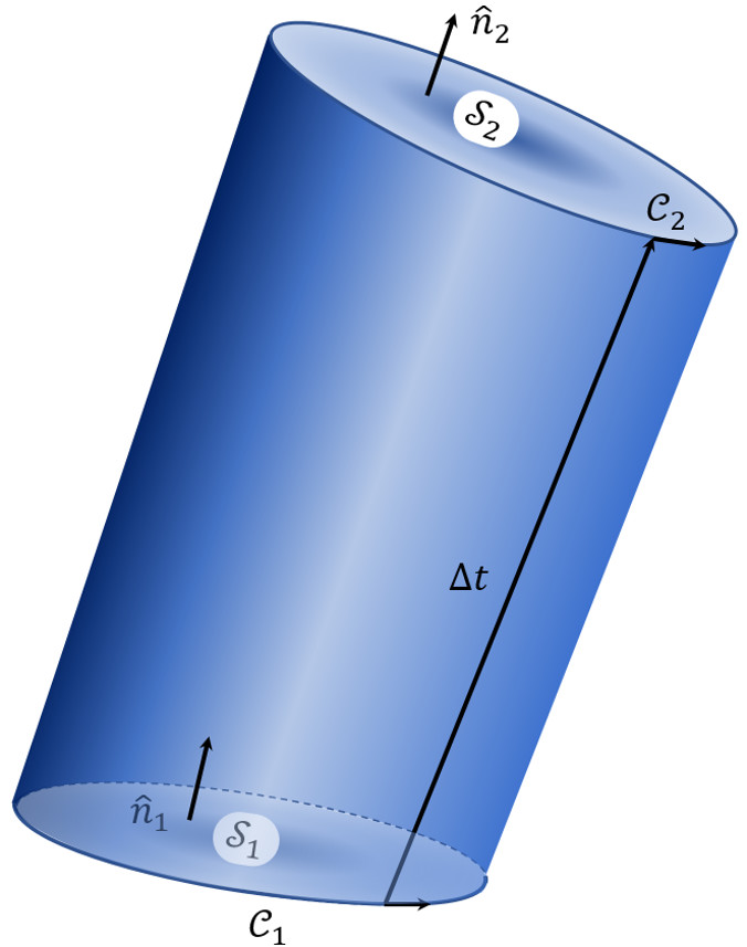
Like a single particle’s trajectory can be thought to trace a path through space, this surface, being two-dimensional, can be thought to trace out a volume, $${\mathcal V}_{total}$$. It is important to remember that to identify the surface’s motion with the volume it crosses, several important changes have to be considered.
First the surface normal on the ‘bottom’ surface must be reversed so that it correspond to the outward normal
\[ \hat n_1 \rightarrow – \hat n_1 \; \]
and that the vector field whose flux is piercing this surface must be evaluated at a common time, which can be arbitrarily chose, without loss of generality, to be $$t_1$$.
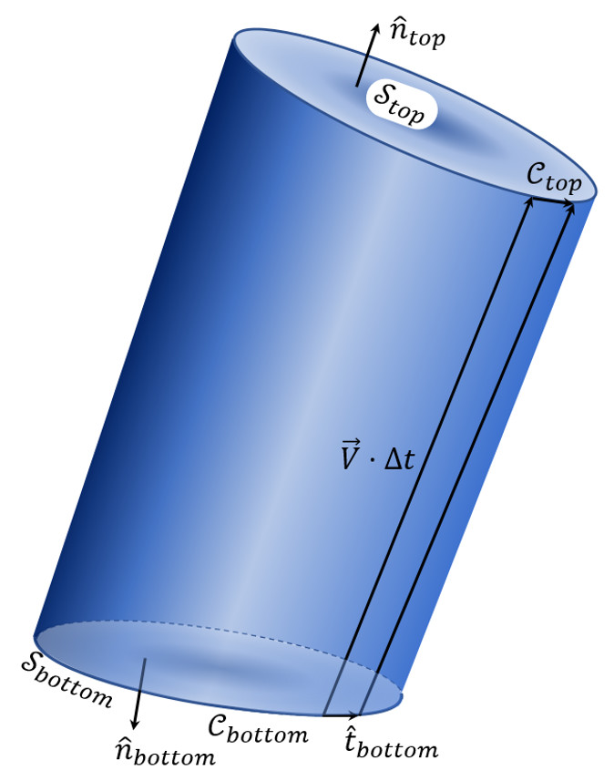
In doing so, the time-varying flux integral has been changed to a volume integral over $${\mathcal V}_{total}$$ at a common time, and the application of the divergence theorem can be used.
The details are as follows. The integral of $$\vec F$$ over the closed surface, $${\mathcal S}_{total}$$ bounding this volume is made of three pieces
\[ \oint_{{\mathcal S}_{total}} d \vec S \cdot \vec F = \int_{top} d \vec S \cdot \vec F + \int_{bottom} d \vec S \cdot \vec F + \int_{side} d \vec S \cdot \vec F \; .\]
The integral over the top surface can be related to the integral over the corresponding surface at time $$t_2$$ by means of the Taylor expansion
\[ \vec F(\vec r, t_2) = \vec F(\vec r, t_1) + \frac{\partial \vec F}{\partial t}(\vec r, t_1) \Delta t + \cdots \; \]
to get
\[ \int_{top} d \vec S \cdot \vec F = \int_{top} d \vec S \cdot \left( \vec F – \frac{\partial \vec F}{\partial t} \Delta t \right) = \int_{{\mathcal S}_2} d \vec S \cdot \left( \vec F – \frac{\partial \vec F}{\partial t} \Delta t \right) \; .\]
The integral over the bottom surface can be related to the integral over the corresponding surface at time $$t_1$$ by means of an overall minus sign reflecting the difference between the volume outward normal and the surface normal
\[ \int_{bottom} d \vec S \cdot \vec F = – \int_{{\mathcal S}_1} d \vec S \cdot \vec F \; .\]
The last piece is the integral over the side. The surface element of the side is
\[ d \vec S_{side} = d\ell \, \hat t \times \vec V \Delta t \; ,\]
where $$\hat t$$ is oriented tangent to $${\mathcal C}_1$$ and $$d \ell$$ is the differential length along it, since this gives the surface area of the parallelogram multiplied by the outward surface normal. The resulting integral is then
\[ \int_{side} d \vec S \cdot \vec F = \int_{{\mathcal C}_1} (d\ell \, \hat t \times \vec V \Delta t) \cdot \vec F = – \int_{side} d\ell \, \hat t \cdot (\vec F \times \vec V \Delta t) \; , \]
where the commutative property of the triple-scalar product was used in the last term.
By the divergence theorem,
\[ \oint_{{\mathcal S}_{total}} d \vec S \cdot \vec F = \int_{{\mathcal V}_{total}} d {\mathcal V}ol \; \nabla \cdot \vec F \; .\]
This latter integral can be further simplified by noting that the volume of any ‘tube’ making up the volume is the area of the base $$d \vec S$$ times (via the scalar product) the height $$\vec V \Delta t$$, giving
\[ d {\mathcal V}ol = d \vec S \cdot \vec V \Delta t \; ,\]
where the surface element is understood to point along $$\hat n_1$$.
The final form of the recast total surface integral is then
\[ \oint_{{\mathcal S}_{total}} d \vec S \cdot \vec F = \int_{{\mathcal S}_{1}} d \vec S \cdot \left( (\nabla \cdot \vec F) \vec V \right) \Delta t \; .\]
Putting the pieces together gives
\[ \int_{{\mathcal S}_{1}} d \vec S \cdot \left( (\nabla \cdot \vec F) \vec V \right) \Delta t = \int_{{\mathcal S}_2} d \vec S \cdot \left( \vec F – \frac{\partial \vec F}{\partial t} \Delta t \right) \\ – \int_{{\mathcal S}_1} d \vec S \cdot \vec F – \int_{{\mathcal C}_1} d\ell \, \hat t \cdot (\vec F \times \vec V \Delta t) \; , \]
where $$\vec F$$ is evaluated at time $$t_1$$ in every term but the first part of the first term on the right-hand side.
Re-arranging the terms results in
\[ \int_{{\mathcal S}_2} d \vec S \cdot \vec F – \int_{{\mathcal S}_1} d \vec S \cdot \vec F = \int_{{\mathcal S}_2} d \vec S \cdot \frac{\partial \vec F}{\partial t} \Delta t \\ + \int_{{\mathcal S}_1} d \vec S \cdot \vec V (\nabla \cdot \vec F) \Delta t + \int_{{\mathcal C}_1} d\ell \, \hat t \cdot (\vec F \times \vec V) \Delta t \; .\]
Dividing the left-hand side by $$\Delta t$$ and taking the limit gives
\[ \lim_{\Delta t \rightarrow 0} \frac{1}{\Delta t} \left( \int_{{\mathcal S}_2} d \vec S \cdot \vec F – \int_{{\mathcal S}_1} d \vec S \cdot \vec F \right) = \frac{d}{dt} \int_{{\mathcal S}_1} d \vec S \cdot \vec F \equiv \frac{d}{dt} \Phi_{\vec F} \; , \]
which is exactly the time derivative of the flux $$\Phi_{\vec F}$$ of $$\vec F$$ through the surface. Thus
\[ \frac{d}{dt} \Phi_{\vec F} = \int_{{\mathcal S}_1} d \vec S \cdot \left( \frac{\partial \vec F}{\partial t} + \vec V (\nabla \cdot \vec F) \right) + \int_{{\mathcal C}_1} d\ell \, \hat t \cdot (\vec F \times \vec V) \; ,\]
where in the limit $${\mathcal S}_2$$ becomes $${\mathcal S}_1$$.
The final step involves recalling that $$t_1$$ was an arbitrary time and so the ‘1’ can be dropped to give
\[ \frac{d}{dt} \Phi_{\vec F} = \int_{{\mathcal S}_t} d \vec S \cdot \left( \frac{\partial \vec F}{\partial t} + \vec V (\nabla \cdot \vec F) \right) + \oint_{{\mathcal C}_t} d\ell \, \hat t \cdot (\vec F \times \vec V) \; .\]
which is the Flux transport theorem in all its glory.