
Continuum Mechanics 6 – Stress and Strain
Up to this point in these posts on continuum mechanics, everything has been generally applicable. The material derivative, the Reynolds and Flux transport theorems, and the nature of the stress tensor are applicable to any type of continuum. Unfortunately, the party needs to end at some point and this post can be considered as the ‘last call’ that signals that end.
To understand why the generalities must stop, we need to discuss something mathematical and something physical.
On the mathematical side, we ultimately need to remind ourselves of a fact that is easy to lose sight of amidst all this machinery. Namely, we are seeking to solve for the behavior of the continuum as a function of time. We are seeking to generalize Newton’s laws to the continuum.
In their conventional setting, Newton’s laws amount to the following statement:
\[ m \frac{d^2 {\bar q}(t)}{d t^2} = {\bar f}({\bar q},{\dot {\bar q}},t) \; , \]
where $$\dot {\bar q}$$ stands for the time-derivative of $${\bar q}(t)$$ as a function of time. The key point here is that the force on the right-hand side, $$\bar f$$ can be determined by knowing the current state itself (state being defined as the phase-space ordered pair of $$({\bar q},{\bar{\dot q}})$$ and time). If this relationship didn’t exist, then literally there would be no way to evolve the system forward in time. Some entity somewhere would need to supply the rule for how to compute the force at each step.
When generalized to a continuum setting, these underlying mathematical requires still hold sway but in a modified form. To give some sense how this modified form might look, consider the wave equation,
\[ \frac{\partial^2 A(x,t)}{\partial t^2} = v^2 \frac{\partial^2 A(x,t)}{\partial x^2} \;, \]
as it is usually presented for the amplitude of a vibrating string $$A(x,t)$$. This equation is usually derived in the continuum limit by looking at a small portion of the string and analyzing the tensions pulling on each side (see, e.g., Mechanics by Symon). The right-hand side of the wave equation is the force on each infinitesimal length of string located at $$x$$. To see this, note that another path to the wave equation uses a discrete, lumped-coupled mass-spring system. This system is then transitioned into a continuum using the appropriate limit as the masses and the spacing between them both go to zero such that ratio of mass to spacing length goes to the mass density. The article on the wave equation in Wikipedia, has an accessible presentation of this latter derivation using discrete masses and springs obeying Hooke’s law.
The point that is again worth emphasizing is that the force on the continuum is known in terms of the continuum itself. Here the state of the system is characterized in terms of the spatial variation of $$A(x,t)$$ through its second partial derivative with respect to $$x$$. This characterization looks odd at first glance but when expressed in terms of finite differences,
\[ \frac{\partial^2 A(x,t)}{\partial x^2} \approx \frac{A(x+h,t) – 2 A(x,t) + A(x-h,t)}{h^2} \; \]
it merely expresses the ‘force’ in terms of the state of the string at points $$x-h, x, x+h$$ and should be considered as no more odd than expressing the force as the combination
\[ \frac{\vec r}{\sqrt{x^2 + y^2 + z^2}} \; \]
as is done for central force laws.
Obviously, what we need to find for continuum mechanics is a relationship that specifies the stress in terms of some function of the state of the continuum. We should prepare ourselves for the fact that the function will almost always depend on some spatial and, perhaps, temporal derivative. We actually got a foretaste of that in the final result of the Reynolds transport theorem
\[ \frac{d}{dt} Vol(t) = Vol(t) div(\vec V) \; , \]
which relates the kinematic description of a small volume to the spatial variation of the flow velocity.
The final step is to sketch out the physical expectations for how that relationship might look functionally for various materials. It is here that the fork in the road comes for which individual materials behave remarkedly different.
In the case of a simple elastic material, the body deforms with an application of a force but returns to its equilibrium shape with the removal of the load. The picture looks something like this:
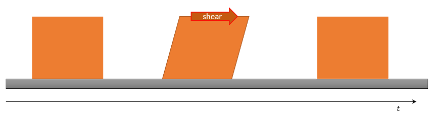
In continuum mechanics, the deformation of the material is described by comparing the initial configuration of the body (usually called the reference configuration) to the configuration after application of the load (usually called the current configuration). The strain of the body (i.e. the response) finds expression in the relative movement of a set of points in the reference configuration to the same set in the current configuration. Removing rigid-body motion leaves what is called the strain. The outcome of this operation is to provide a direct functional connection $$\sigma = f(\epsilon)$$ between the observed strain, $$\epsilon$$, and the applied stress, $$\sigma$$, which is what is needed to have mathematical closure. This relationship generalizes the usual Hooke’s law encountered in basic mechanics, which states that the force due to a spring is given by $$\vec F = -k \vec x$$, but the generalization, although still linear, is a bit more complicated due to tensorial nature of the stress and strain.
In contrast to elastic materials, whose deformation only persists as long as the stress is applied, fluids (liquids and gases) flow under the application of a stress. Their deformations continue to change after the load is removed.
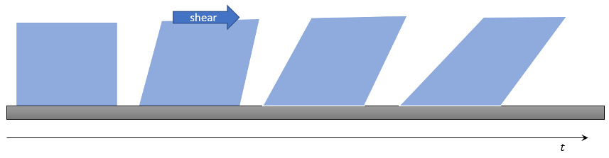
In these cases, the key observation comes from Newtonians laws. The stress being an outside force, can only accelerate the material during its application. The key relationship that relates the stress to an observed property of the body is of the form $$\sigma = f(\dot \epsilon)$$, which says that by observing the rate-of-change of the strain one can deduce the stress-applied.
To be complete, the two relationships detailed above only scratch the surface of the various types of materials and the resulting functional relationships between strain in a body and the stress applied. There are hosts of other behaviors and often the situation is muddled due to the fact that the functional relationship is determined ‘the other way around’. New materials are subjected to a variety of known stresses in order to observe the corresponding strains. This approach results in an implicit relationship between strain and stress. But regardless of whether the relationship is explicit or implicit, the mathematical closure of the theory requires that the force on the material be expressible as a function of the state of the material and, perhaps time, just as it is done for ordinary particle mechanics.
The coming posts will explore some of these relationships explicitly but no attempt to be complete and comprehensive will be made – nature is just too varied to believe that can be done.