
Continuum Mechanics 7 – Elastic Strain Basics
As part of the series on Continuum Mechanics, this post is the first of several focusing on elastic behavior of materials. Referring to the previous post, elastic materials are ones which, in contrast with fluids, deform under the application of a stress but return to their equilibrium shape upon the removal of the stress.
Before characterizing the strain mathematically, consider first some physical expectations from the simple bending of a beam under the load. To focus the discussion, look at the three specific points in orange, yellow, and black.
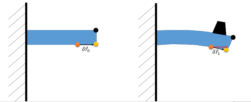
Prior to the deformation, the separation between the orange and yellow points is entirely along the horizontal, and the separation between the yellow and black points is entirely along the vertical. Denote the relative position of the orange point relative to the yellow as $$\delta {\vec r}_0$$ and then examine what happens to that relative position under a load. When the beam bends, the material along the top edge stretches while the material along the bottom compresses. This is seen by the fact that the new relative position, $$\delta {\vec r}_1$$, from orange to yellow is now shorter in length and has components in both directions (its original length and direction being shown in red). Likewise, the relative position between yellow and black changes its orientation substantially but negligibly changes its length since both points are along the edge and the bending stress barely compresses the material at the edge.
The deformation of the relative position from the orange and yellow points measures how much change $$\delta {\vec r}_0$$ suffers under the load of the bending stress. Care needs to be exercised when examining the change in orientation since a rigid body rotation does not constitute deformation even though it rotates the entire body. Thus, the measure of deformation should look something like
\[ deformation = \delta {\vec r}_1 – \delta {\vec r}_2 – rigid\;\;body\;\;rotations \; ,\]
with the additional understanding that this deformation will vary from point to point within the material, that is, the deformation is a field.
The mathematical characterization of deformation presented here closely follows Mathematical Methods for Physicists by Arfken, Third Edition.
Like the bending beam discussed above, Arfken focuses on two points at $${\mathcal P}_0$$ and $${\mathcal Q}_0$$.
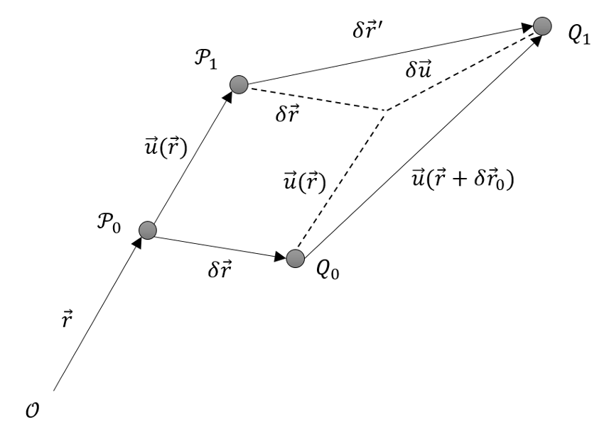
Assume $${\mathcal P}_0$$ is located at $${\vec r}$$ and that the relative position of $${\mathcal Q}_0$$ is $$\delta {\vec r}$$. Under the applied stress, $${\mathcal P}_0$$ transports by $${\vec u}(\vec r)$$ to its new location at $${\mathcal P}_1$$. Likewise, $${\mathcal Q}_0$$ transports by $${\vec u}(\vec r + \delta {\vec r})$$ to its new location $$\delta {\vec r}’ = {\vec u} + \delta {\vec u}$$ relative to $${\mathcal P}_1$$. Because it describes the transport of each point in the material, $${\vec u}({\vec r})$$ is called the transport field.
Since a rigid-body motion would have transported both $${\mathcal P}_0$$ and $${\mathcal Q}_0$$ by a common $${\vec u}$$, independent of position, the deformation is clearly related to any transport difference, $$\delta {\vec u}$$, between the two.
The transport difference
\[ \delta {\vec u}({\vec r}) = {\vec u}({\vec r}+\delta {\vec r}) – {\vec u}({\vec r}) \; \]
expands, to first order, as
\[ \delta {\vec u} = \nabla_{\vec r} {\vec u} \cdot {\vec r} \; .\]
The gradient of the transport field is a second-rank tensor, called the transport tensor, that maps an initial relative position to a final transport difference. In components, its representation is
\[ \nabla {\vec u} = \frac{\partial u_i}{\partial r_j} \delta r_j \equiv \partial_j u_i \delta r_j \; . \]
It is important to realize that $$\nabla {\vec u}$$ is not yet the strain tensor being hunted. There is a possibility that there is a rotation hidden within.
The usual way to deal with this is to decompose the transport tensor into symmetric and anti-symmetric pieces defined through
\[ \delta u_i = \eta_{ij} \delta r_j + \xi_{ij} \delta r_j \; , \]
where
\[ \eta_{ij} = \frac{1}{2} \left( \partial_j u_i + \partial_i u_j \right) \, \]
and
\[ \xi_{ij} = \frac{1}{2} \left( \partial_j u_i – \partial_i u_j \right) \, . \]
Arfken notes that the anti-symmetric piece, which is related to the curl of the transport field, contains the rigid-body rotations. To see this, consider the following expression
\[ [ (\nabla \times {\vec u}) \times \delta {\vec r} ]_i = \epsilon_{ijk} \epsilon_{j\ell m} \partial_{\ell} u_m \delta r_k \; , \]
where $$[{\vec r}]_j \equiv r_j$$ is the jth component of the vector $${\vec r}$$.
Performing the usual index gymnastics yields
\[ [ (\nabla \times {\vec u}) \times \delta {\vec r} ]_i = \partial_j u_i \delta r_j – \partial_i u_j \delta r_j = 2 \xi_{ij} \delta r_j \; . \]
So the anti-symmetric portion of the transport difference represents a rotation of $${\mathcal Q}$$ about $${\mathcal P}$$ along the $$\nabla \times {\vec u}$$ axis by $$|\nabla \times {\vec u}|$$ radians.
The symmetric piece of the transport difference, $$\eta_{ij}$$, represents the actual strain that develops at $${\vec r}$$.
The diagonal components of $$\eta_{ij}$$ represent stretches or compressions and the off-diagonal components correspond to shears. To see these assertions consider the original orange and yellow points separated from each other by one unit of distance along the horizontal, which, for convenience, will be called the x-axis: ($$\delta {\vec x} = {\hat \imath} $$).
After the deformation, the transport difference is given by
\[ \delta {\vec u} = \eta_{11} {\hat \imath} + \eta_{12} {\hat \jmath} + \eta_{13} {\hat k} \; .\]
The position of yellow relative to orange is given by
\[ \delta {\vec y} = \delta {\vec x} + \delta {\vec u} = (1 + \eta_{11} ) {\hat \imath} + \eta_{12} {\hat \jmath} + \eta_{13} {\hat k} \; .\]
Projected into two dimensions, the before and after configurations look as below.
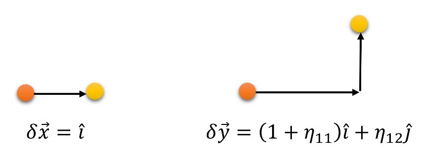
Note that the change in the relative position has components along both the $$x$$- and $$y$$-axes, with the later growing larger as the distance along the $$x$$-axes from the orange point grows. Since the length of the relative position changed, there is a scaling involved. Also, the growth along the $$x$$-axis of the vertical component represents a shear in contrast to a rotation.
With the basic notions of the strain tensor $$\eta_{ij}$$ well established, the next post will cover the mapping of this tensor to the various moduli of elasticity.