
Continuum Mechanics 8 – Elastic Moduli
The last post introduced the idea of the deformation field $${\vec u}(\vec r)$$ and the corresponding strain tensor $$2\epsilon_{ij} = \partial_j u_i + \partial_i u_j$$, which characterizes the amount that any two points in the continuum move away from each other.
While formally correct, the mathematical form of the strain tensor tends to obscure any physical intuition as to what different components are all about. Some small hint for how to interpret the strain tensor was touched upon in the closing of the last post. This post provides a more in-depth coverage by introducing the elastic moduli.
The elastic moduli generalize the concept of a spring concept from elementary mechanics. Roughly speaking, these numbers describe the resistance that the material has to one of three basic actions: 1) Young’s modulus (usually called $$E$$) – being stretched or compressed along a particular direction, 2) bulk modulus (usually called $$K$$) – being expanded or contracted in all directions, and 3) shear modulus (usually called $$G$$) – being sheared. The primary distinction between 1) and 2) is that the density of the material need not change during a uniaxial deformation but must necessarily change for a full expansion or contraction. Detail for each of these follows.
Youngs Modulus
Consider a uniform rod of material of a rectangular cross-section $$A$$ with a natural length (i.e. stress-free) $$L$$. When subjected to a tension force $$F$$, the rod expands by $$\Delta L$$.
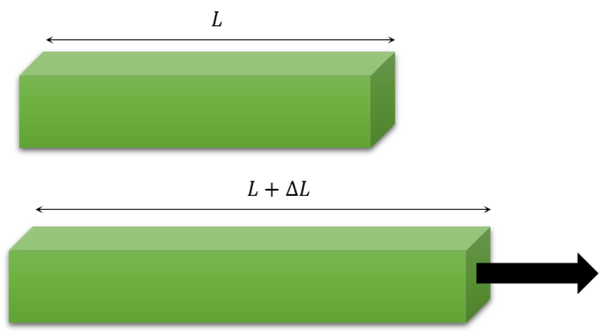
Measurements of the extent of the stretch as a function of the stress gives Young’s modulus as
\[ E = \frac{F/A}{\Delta L/L} = \frac{T_{xx}}{\epsilon_{xx}} \; , \]
where the last equality follows by defining the long axis of the bar as the $$x$$-axis and $$T_{xx}$$ and $$\epsilon_{xx}$$ are the corresponding components of the stress and strain tensors.
Interestingly, the story of uniaxial stress isn’t quite complete. As anyone who has every play with rubber bands knows, when an elastic material lengthens in one direction it typically shrinks in the transverse directions; the band gets thinner in the two directions perpendicular to the ‘stretch’ direction.
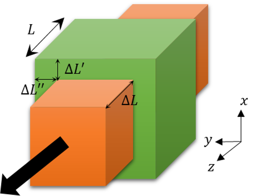
Generally, the transverse directions do not shrink by the same amount since the degree of contraction depends on material composition and this difference is manifest in $$\Delta L’ \neq \Delta L”$$. Poisson’s ratios are defined as
\[ \nu_{zx} = -\frac{\Delta L’}{\Delta L} \; \]
and
\[ \nu_{zy} = -\frac{\Delta L”}{\Delta L} \; ,\]
where the notation $$\nu_{ij}$$ measures the ratio of change along the $$j$$-axis as a function of the strain caused along the $$i$$-axis by the corresponding stress.
When $$\Delta L’ = \Delta L”$$ the material has an axis of symmetry about which there is an axial uniformity. If Young’s modulus is the same in all direction, then the material is called isotropic and no indices are needed as there is only one Poisson’s ratio needed. The assumption of isotropy works for many simple materials but certain elastic man-made materials have very directionally-dependent Poisson ratios. The Wikipedia article on Poisson’s ratio lists six separate ratios $$\nu_{ij}$$ for the fabric Nomex.
Note that as the material undergoes its elongation and retraction in the direction of the stress and in the perpendicular directions, respectively, that the density can remain constant or that it change. The exact determination depends on the material as does just how much the two perpendicular directions differ in the amount they contract.
Bulk Modulus
Consider a small unit of material suddenly placed inside a high-pressure environment. An example would be the submergence of a metal cube at the bottom of the ocean. Compression stress assaults the cube from all sides seeking to change the volume and, hence, the density of the material.
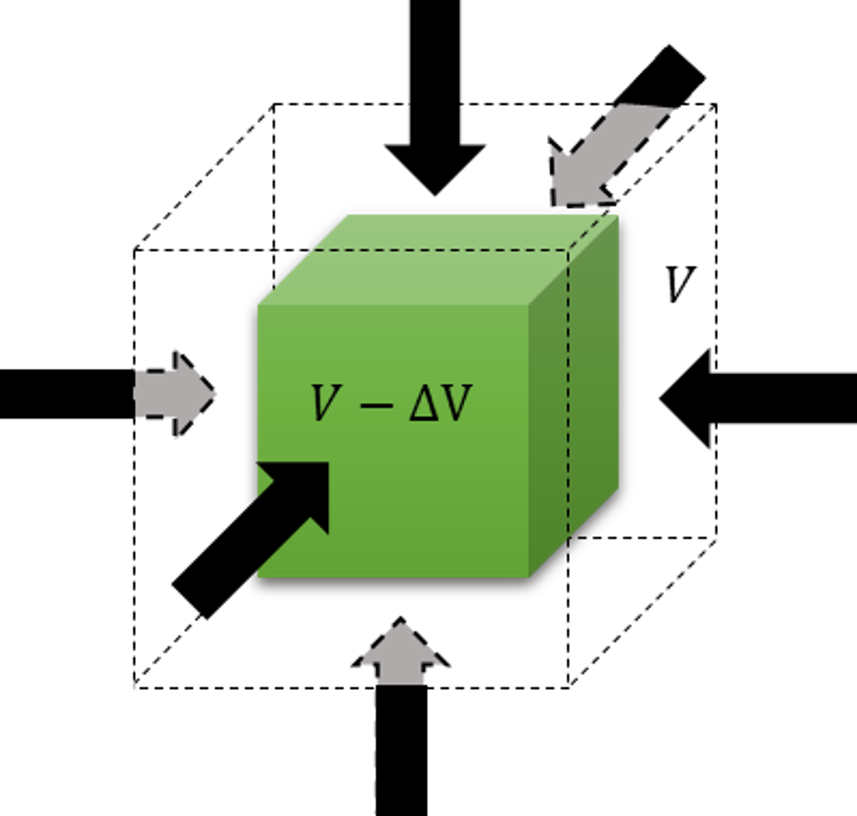
The bulk modulus measures how resistant the material is to this change and, defined as the ratio of the pressure $$P$$ to the fractional change in the volume $$\Delta V / V$$, becomes
\[ K = – \frac{\Delta P}{\Delta V/V} \approx -V \frac{d P}{d V} ; .\]
Shear Modulus
Consider a rod of material that is placed between two plates, the bottom one fixed and the top one free to move along the $$x$$-direction. As it moves, the top plate exerts a stress $$T_{xy}$$ on the top face of area $$A$$, which deforms the material by varying degrees as a function of distance $$y$$ from the fixed plate.
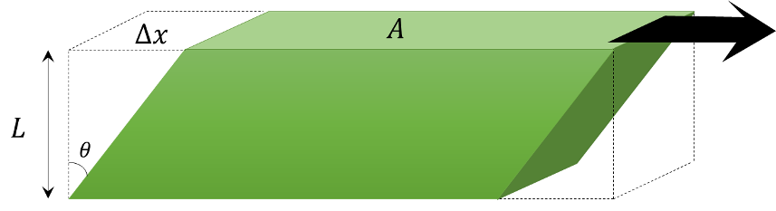
If the height of the rod is $$L$$ and the amount of deformation at the top is $$\Delta x$$ then the shear modulus is defined as
\[ G_{xy} = \frac{F/A}{\Delta x/L} = \frac{T_{xy}}{\partial_y u_{x}} = \frac{T_{xy}}{2 \epsilon_{xy}} \; . \]
Similar expressions exist for the other possible combinations of directions. An isotropic material needs only one shear modulus to describe it.
General Relation of Strain to Stress
The definitions of the three basic moduli relate strain to stress in an intuitive and geometric way but the tensor nature of the stress and strain are absent and any connection between the moduli are obscure at this point. The final step is to synthesize them into a general relationship between the stress tensor $$T_{ij}$$ and the strain relationship $$2 \epsilon_{ij}$$ and to discover how the moduli connect to each other.
The full tensor relationship is given by the generalize Hooke’s law
\[ T_{ij} = c_{ijkl} \epsilon_{kl} \; , \]
where the fourth-rank stiffness tensor $$c_{ijkl}$$ plays the role of the spring constant in the simply form of Hooke’s law $$F = -k x$$. There are 81 different components of the stiffness tensor but most of them are not independent. The symmetric nature of the stress and strain tensors ($$T_{ij} = T_{ji}$$ and $$\epsilon_{ij} = \epsilon_{ji}$$) imposes the relationships
\[ c_{ijkl} = c_{jikl} = c_{ijlk} = c_{jilk} \]
reducing the number of independent components to 36. A further reduction down to 21 independent components comes from noting that the stiffness matrix is also symmetric upon the interchange of the first and second pair of indices
\[ c_{ijkl} = c_{klij} \; .\]
This symmetry in the stiffness tensor is inherited from the potential energy for an elastic body
\[ PE = \frac{1}{2} c_{ijkl} \epsilon_{ij} \epsilon_{kl} \; , \]
which is clearly invariant under the exchange of $$\epsilon_{ij}$$ and $$\epsilon_{kl}$$.
Next month’s column focuses on isotropic materials, exploring the specific relationships between the moduli in this case, and by looking at how elastic waves propagate.