
Continuum Mechanics 10 – Tying Up Loose Ends
This month’s post marks the end of the study of continuum mechanics, or rather it marks the end of the name. The past nine posts have focused on the basic material common to elasticity and fluids and then moved into a brief study of elastic motion. The material here will serve as the final post on elasticity, cleaning up some loose ends and providing some rigor. Next month, the focus will turn to fluid mechanics and the series will be retitled and renumbered accordingly.
The three topics covered here provide some additional details and rigor to the discussions that have come before with a particular focus on the elastic equations of motion that are used to analyze the wave motion discussed in post 9.
Rigorous derivation of the strain tensor
When I was first exposed to elasticity, it was from Chapter 3 of Mathematical Methods, 3rd edition by Arfken; and, in fact, I used that text as a guide for the material in post 7. However, a brief consultation with more specialized texts will often yield a strain tensor that is a bit more complex than the one presented in either of those two sources. A more complete derivation, which is patterned after the derivation here, supplemented with my own insights, is as follows.
Let the position of any point at any stage of the deformation be defined by $${\vec r}_t = \vec \phi (\vec r, t)$$, where $$\vec r$$ is the initial position of the point and $$t$$ measures the extent of deformation. The function $$\vec \phi(\vec r,t)$$ is called the flow mapping. The parameter $$t$$ parameterizes the deformation, labeling the successive stages. It doesn’t necessarily need to be regarded as the time but it is often convenient to treat it as such and it will used that way below. The requirement that $$\vec r$$ is the original undeformed position imposes the obvious boundary: $$\vec \phi (\vec r, 0) = \vec r$$.
Now focus on two points $${\mathcal P}$$ and $${\mathcal Q}$$ before and after the derivation. Their positions before the deformation are:
\[ \vec {\mathcal P}(0) = \vec \phi(\vec r,0) = \vec r \; \]
and
\[ \vec {\mathcal Q}(0) = \vec \phi(\vec r + d \vec r,0) = \vec r + d \vec r \; . \]
After the deformation, the same two points are now located at
\[ \vec {\mathcal P}(t) = \vec \phi(\vec r, t) \; \]
and
\[ \vec {\mathcal Q}(t) = \vec \phi(\vec r + d \vec r,t) = \vec \phi(\vec r,t) + \frac{\partial \vec \phi(\vec r, \epsilon) }{\partial \vec r} d \vec r \; , \]
where the assumptions that $$d \vec r$$ is small in magnitude and that $$\vec \phi$$ is differentiable have been made.
Now measure the distance between the points $${\mathcal P}$$ and $${\mathcal Q}$$. Before the deformation, that distance squared is given by
\[ ds^2 = \left\Vert \vec {\mathcal P}(0) – \vec {\mathcal Q}(0) \right \Vert^2 = d \vec r \cdot d \vec r = d r_i d r_i \; . \]
After the deformation, the distance squared between those points, now moved to their new position, is given by
\[ ds_{t}^2 = \left\Vert \vec {\mathcal P}(t) – \vec {\mathcal Q}(t) \right \Vert^2 = \frac{\partial \phi_i}{\partial r_j} d r_j \frac{\partial \phi_i}{\partial r_k} d r_k \; . \]
Calculate the difference between these two lengths
\[ ds_{t}^2 – ds^2 = \frac{\partial \phi_i}{\partial r_j} d r_j \frac{\partial \phi_i}{\partial r_k} d r_k – d r_j d r_k \delta_{jk} = \left( \frac{\partial \phi_i}{\partial r_j} \frac{\partial \phi_i}{\partial r_k} – \delta_{jk} \right) dr_j dr_k\; ,\]
where the last term has been modified a bit by the inclusion of a Kronecker delta.
We now define the Green-Lagrange strain tensor by the relationship
\[ 2 \epsilon_{jk} = \frac{\partial \phi_i}{\partial r_j} \frac{\partial \phi_i}{\partial r_k} – \delta_{jk} \; .\]
The strain vector $$\vec u$$ measures the difference in position between where a particle originally was located and where it is located at time $$t$$
\[ \vec u(t) = \vec \phi(\vec r,t) – \vec r \; . \]
Spatial derivatives of $$\vec \phi$$ are related to spatial derivatives of the deformation vector $$u$$ via
\[ \frac{\partial \phi_i(\vec r,t)}{\partial r_j} = \delta_{ij} + \frac{\partial u_i}{\partial r_j} \; . \]
Substituting this expression into the Green-Lagrange strain tensor gives
\[ 2 \epsilon_{jk} = \left( \delta_{ij} + \frac{\partial u_i}{\partial r_j} \right) \left( \delta_{ik} + \frac{\partial u_i}{\partial r_k} \right) – \delta_{jk} \; . \]
Expanding and simplifying yields
\[ \epsilon_{jk} = \frac{1}{2} \left( \frac{\partial u_k}{\partial r_j} + \frac{\partial u_j}{\partial r_k} + \frac{\partial u_i}{\partial r_j}\frac{\partial u_i}{\partial r_k} \right) \; , \]
which is the same as the earlier derivation except for the nonlinear term that can often be dropped.
Rigorous derivation of the equations of motion
The same notions can be used to derive the equations of motion that led to the wave equation analyzed in the last post. Consider a cube of the continuum centered at $$\vec r$$.
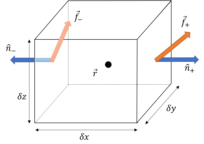
The force on any face is given by $$f_i = T_{ij} n_j Area$$. Start first with the forces on the two faces perpendicular to the $$x$$-axis. The center of the rightmost face is located at $$\vec r + (\delta x/2) \hat \imath$$ and it is at this point that the stress is evaluated. Likewise, the center of the leftmost face lies at $$\vec r – (\delta x/2) \hat \imath$$. For notational convenience, functions evaluated on the rightmost face will be denoted with the argument $$x_{+}$$ and those evaluated on the leftmost face with $$x_{-}$$. In this notation, the components of the forces on these faces are:
\[ \left[ \begin{array}{c} f_x \\ f_y \\ f_z \end{array} \right] = \left[ \begin{array}{c} T_{xx}(x_+) – T_{xx}(x_-) \\ T_{yx}(x_+) – T_{yx}(x_-) \\ T_{zx}(x_+) – T_{zx}(x_-) \end{array} \right] dy dz = \left[ \begin{array}{c} T_{xx,x}(\vec r) \\ T_{yx,x}(\vec r) \\ T_{zx,x}(\vec r) \end{array} \right] dx dy dz \; , \]
where the last equalities result by taking a Taylor’s expansion of the finite difference and keeping terms of only first order ($$T_{ij,k} = \partial T_{ij} / \partial r_k$$).
Similar manipulations give the expressions
\[ \left[ \begin{array}{c} f_x \\ f_y \\ f_z \end{array} \right] = \left[ \begin{array}{c} T_{xy}(y_{+}) – T_{xy}(y_-) \\ T_{yy}(y_+) – T_{yy}(y_-) \\ T_{zy}(y_+) – T_{zy}(y_-) \end{array} \right] dx dz = \left[ \begin{array}{c} T_{xy,y}(\vec r) \\ T_{yy,y}(\vec r) \\ T_{zy,y}(\vec r) \end{array} \right] dx dy dz \; \]
and
\[ \left[ \begin{array}{c} f_x \\ f_y \\ f_z \end{array} \right] = \left[ \begin{array}{c} T_{xz}(z_+) – T_{xz}(z_-) \\ T_{yz}(z_+) – T_{yz}(z_-) \\ T_{zz}(z_+) – T_{zz}(z_-) \end{array} \right] dx dy = \left[ \begin{array}{c} T_{xz,z}(\vec r) \\ T_{yz,z}(\vec r) \\ T_{zz,z}(\vec r) \end{array} \right] dx dy dz \; , \]
for the components of the force generated on the $$y$$- and $$z$$-faces, respectively.
Combining these results and expressing the sums in index notation gives the final, compact expression for the force as
\[ f_i = T_{ij,j} dx dy dz \; .\]
Note that the mass of the continuum contained in the cube is $$\rho \, dx dy dz$$, where $$\rho$$ is the mass density. Newton’s second law for the cube then relates the acceleration of the cube, which is expressed in terms of the second time-derivative of the flow mapping to the cube’s mass and the forces acting on the cube as
\[ (\rho \, dx dy dz) \frac{\partial^2 \phi(\vec r,t)}{\partial t^2} = f_i \; . \]
Using the relation between the flow mapping and the deformation vector and between the force and the stress tensor gives
\[ \rho \, \partial^2_t u_i = T_{ij,j} \; , \]
which is precisely the starting expression for the last post.
Relation between the Lame constants and the elastic moduli
This final section derives the relationships to express the elastic moduli derived in post 7 to the Lame constants, which were introduced as a shorthand for the wave equation in an isotropic medium. The Lame constants took the form
\[ \lambda = \frac{\nu E}{(1+\nu)(1-2\nu)} \; \]
and
\[ \mu \frac{E}{2(1+\nu)} \; ,\]
where $$E$$ is Young’s modulus and $$\nu$$ is Poisson’s ratio.
It is a matter of some simple algebra to express Young’s modulus and Poisson’s ration in terms of $$\lambda$$ and $$\mu$$ as follows. Manipulating the second equation gives $$E = 2 (1+\nu) \mu$$. Substituting this into the first equation gives $$\lambda = 2 \nu \mu / (1-2\nu)$$ from which one gets via simplification
\[ \nu = \frac{\lambda}{2 (\mu + \lambda) } \; . \]
Back-substituting gives
\[ E = \mu \frac{2\mu + 3 \lambda}{\mu + \lambda} \; \]
for Young’s modulus.
To relate the shear and bulk moduli to the Lame constants, return to the generalized Hooke’s law
\[ T_{ij} = 2 \mu \epsilon_{ij} + \lambda Tr(\epsilon) \delta_{ij} \; . \]
In the case of an isolated shear along the $$x$$-direction that grows along the $$y$$-direction, the strain is expressed as $$\partial_y u_x$$ and the only non-zero terms in the strain tensor are $$ \epsilon_{xy} = \epsilon_{yx} = 1/2 \, \partial_y u_x$$. Thus,
\[ T_{xy} = 2 \mu \epsilon_{xy} = 2 \mu \frac{1}{2} \partial_y u_x = \mu \partial_y u_x \; .\]
Since the shear modulus is defined (see post 8) as the ratio of stress $$T_{xy}$$ and the strain $$\partial_y u_x$$, it is clear that $$G = \mu$$.
Finally, the bulk modulus applies when the continuum is in isotropic (i.e. hydrostatic) stress equilibrium. Isotropic stress means that the strain tensor is diagonal with all its on-diagonal components equal: $$T_{xx} = T_{yy} = T_{zz} \equiv T_{iso}$$. The strain tensor is also diagonal with $$\epsilon_{xx} = \epsilon_{yy} = \epsilon_{zz} \equiv \epsilon_{iso}$$. The application of $$T_{iso}$$ represents a pressure that uniformly compresses the continuum. The measure of that compression is given by the fractional change in volume. Consider a small cube of initial length $$L$$ on a side so that applying $$T_{iso}$$ causes an isotropic strain of $$\Delta L$$ in all directions. The volume before the strain is $$L^3$$ and the volume after is, to first order, $$L^3 – 3 L^2 \Delta L$$. The fractional change in the volume is then
\[ \frac{\Delta V}{V} = -\frac{3 L^2 \Delta L}{L^3} = -3 \frac{\Delta L}{L} = -3 \epsilon_{iso} \; . \]
The bulk modulus is defined as the ratio
\[ K = -\frac{\Delta P}{\Delta V/V} = \frac{T_{iso}}{3 \epsilon_{iso}} \; .\]
From the generalize Hooke’s law
\[ T_{iso} = 2 \mu \epsilon_{iso} + \lambda 3 \epsilon_{iso} = (2 \mu + 3 \lambda) \epsilon_{iso} \; . \]
Comparing the two expressions gives
\[ K = \lambda + \frac{2}{3} \mu \; . \]
So, that’s it for now on elastic solids and that corner of continuum mechanics. Next month, I turn towards the related subdiscipline of fluid mechanics.