
Bernoulli’s Principle
The Navier-Stokes equation derived in the previous post represents a springboard for the study of Newtonian fluids in a variety of scenarios. Because of the complexity of the equations of fluid mechanics, even this ‘approximation’ represents a degree of complexity that has yet to be completely understood. In fact, questions about the structure and existence of solutions to the Navier-Stokes equations are considered to be so important that the Clay Mathematics Institute is offering a Millennium Prize for proofs associated with this system as a step towards understanding turbulence.
As a result, the next set of posts will focus on subsets of these equations with the examples often being even more simplified. The hope is by looking at simple scenarios a degree of intuition may be developed. This approach is largely influenced by the fine book Elementary Fluid Mechanics by Acheson.
The first block of these will be concerned with the original jewel in the mathematical modeling of fluids in the 18th and 19th centuries – an ideal fluid.
An ideal fluid is a drastic simplification to the fluid flow model in which internal transports of energy or momentum between fluid elements are ignored. Thus the internal energy of a fluid element remains constant during the flow and its kinetic energy and momentum change only due to the external forces. In addition, the flow is assumed to be incompressible ($$\nabla \cdot \vec V = 0$$), meaning that the density of any fluid element remains constant during the flow and, as a further simplification, each fluid element will be assigned the same value of density. Note that these are two distinct assumptions about the density, a point Acheson goes to great lengths to emphasize in his discussion on pages 6, 23-4, and, in particular, 356, where he states quite clearly that:
Despite these seemingly drastic simplifications, there are numerous ordinary, terrestrial applications of the theory. The most common one would be the flow of water in a variety of ‘household’ circumstances. It should be noted that the assumption of incompressibility and a constant, homogeneous density is actually a better assumption than that the fluid has no viscosity (i.e. is inviscid). Fluid compressibility needs to be more carefully considered only when the flow speeds near the speed of sound in the fluid. Nonetheless, the ideal fluid was the jewel of yesteryear mostly because these assumptions actually meant one could solve a problem, even if the problem only partially matched what was physically observed. This gap between what can be modeled and what is observed will become a common theme in the posts to follow.
To get the equations for an ideal fluid, start with the Navier-Stokes equations
\[ \rho \frac{D \vec V}{D t} = – \nabla P + \mu^2 \nabla \vec V + \frac{1}{3} \mu \nabla (\nabla \cdot \vec V) + \rho \vec g \; , \]
(where the material derivative $$D/Dt = \partial_t + \vec V \cdot \nabla$$), and set the viscosity $$\mu$$ equal to zero, yielding Euler’s equations
\[ \frac{D \vec V}{dt} = -\frac{1}{\rho} \nabla P + \vec g \; .\]
In addition to these equations, we always have the continuity equation
\[ \frac{D \rho}{d t} + \rho \nabla \cdot \vec V = 0 \; ,\]
which, given the two incompressibility assumptions, simplifies to
\[ \nabla \cdot \vec V = 0 \; \]
and
\[ \rho = \mathrm{constant} \; .\]
Taken together, these are a set of 4 equations in the 4 unknowns $$\vec V$$ and $$P$$ (with $$\rho$$ assumed to be known for the particular situation).
Even in this simple form, the equations can be quite hard to solve as can be more readily seen if the equations are put into component form (after expanding the material derivative):
\[ \partial_t V_x + V_x \partial_x V_x + V_y \partial_y V_x + V_z \partial_z V_x = – \frac{1}{\rho} \partial_x P \; ,\]
\[ \partial_t V_y + V_x \partial_x V_y + V_y \partial_y V_y + V_z \partial_z V_y = – \frac{1}{\rho} \partial_y P \; ,\]
\[ \partial_t V_z + V_x \partial_x V_z + V_y \partial_y V_z + V_z \partial_z V_z = – \frac{1}{\rho} \partial_z P \; ,\]
and
\[ \partial_x V_x + \partial_y V_y + \partial_z V_z = 0 \; .\]
Obviously, these equations are not particularly illuminating, even for the great masters of the 18th and 19th centuries. It is remarkable then, that there is a very convenient simplification that was discovered by Daniel Bernoulli, called Bernoulli’s principle, which he published in 1738.
While Bernoulli didn’t have access to modern vector calculus (making his discovery all the more remarkable), we will not be too proud to employ it since it will make the derivation clearer and will serve as a springboard to subsequent discoveries.
Return to Euler’s equation
\[ \partial_t \vec V + (\vec V \cdot \nabla) \vec V = -\frac{1}{\rho} \nabla P + \vec g \; .\]
The most troublesome term is the nonlinear $$(\vec V \cdot \nabla) \vec V$$ term on the left-hand side. A convenient vector identity can be employed to separate this nonlinear term into solenoidal and irrotational pieces
\[ (\vec V \cdot \nabla) \vec V = (\nabla \times \vec V) \times \vec V + \nabla \left( \frac{1}{2} \vec V^2 \right) \].
We know define the vorticity vector (more about this in the next post) as
\[ \vec \omega = \nabla \times \vec V \; .\]
Euler’s equation now becomes (moving the irrotational term to the right-hand side)
\[ \partial_t \vec V + \vec \omega \times \vec V = -\nabla \left( \frac{1}{2} \vec V^2 \right) -\frac{1}{\rho} \nabla P + \vec g \; .\]
Since the gravitational force can also be derived from the gradient of a potential $$\vec g = -\nabla \chi$$, Euler’s equation can finally be written as
\[ \partial_t \vec V + \vec \omega \times \vec V = -\nabla H \; , \]
where
\[ H = \frac{P}{\rho} + \chi + \frac{1}{2} \vec V^2 \; \]
Now if the flow is steady, the time variation can be set to zero. Taking the dot product of both sides with $$\vec V$$ and noting that $$\vec V \cdot (\vec \omega \times \vec V) = \omega \cdot (\vec V \times \vec V) = 0$$ yields
\[ \vec V \cdot (\nabla H) = (\vec V \cdot \nabla) H = 0 \; .\]
The physical interpretation of this equation is that the value of H is conserved, for a given fluid element, as it flows. This, then, is Bernoulli’s principle which states that changes of a fluid element’s flow speed are balanced by corresponding changes in pressure or gravitational potential energy, such that the initial value of H remains constant.
Bernoulli’s principle precisely describes how high flow from a faucet, a garden hose, or fountain can reach when pushed upward from an orifice when it emerges with a particular pressure and speed. It represents the simplest form of energy conservation for a fluid.
A simple example of the Venturi tube will illustrate some of the applications. Consider the pipe shown below (assume cylindrical symmetry).
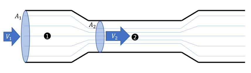
Let the inlet area and speed be $$A_1$$ and $$V_1$$, respectively, and the area and speed at the middle of the pipe be $$A_2$$ and $$V_2$$. The question we can answer is what is the difference between the inlet pressure and the pressure at the center. Following any stream line (thin blue lines), we know that the mass of the fluid element is conserved and so the total inlet mass must be conserved. The continuity equation takes the form
\[ \rho_1 A_1 V_1 = \rho_2 A_2 V_2 \; , \]
for mass per unit time.
Using Bernoulli’s equation we also get
\[ \frac{P_1}{\rho_1} + \frac{1}{2} V_1^2 = \frac{P_2}{\rho_2} + \frac{1}{2} V_2^2 \; .\]
Now, for an ideal fluid, the density is constant, and we can solve for $$V_2$$ in terms of the known areas and inlet speed. Substituting this result in Bernoulli’s gives a pressure difference of
\[ P_1 – P_2 = \frac{1}{2} \rho V_1^2 \left[ \left( \frac{A_1}{A_2} \right)^2 – 1 \right] \; \]
Clearly showing that the pressure at the center of the tube is lower than at the inlet with the difference depending on the inlet speed and the ratio of the two cross-sectional areas. This tube is used in the Venturi meter to determine/monitor flow speeds.
Next post will examine the role that the vorticity plays in ideal fluid flow.