
Vorticity
The last post developed the basic theory of an ideal fluid, teased out Bernoulli’s theorem, and introduced the concept of fluid vorticity. While these basic results are fairly simple there are certain caveats that need to be observed and applications of this theory can be tricky if they are not. To illustrate some of the complexities that can arise when careful thinking is not exercised, this post considers the rotating bucket problem discussed in Acheson’s Elementary Fluid Dynamics.
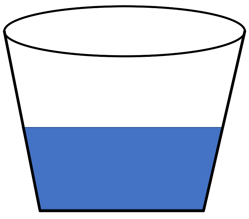
To begin, start with the simpler physical situation with the bucket filled with water that is sitting quietly on a table. The free surface of the water has a flat profile whose normal is parallel with the vertical, a configuration that is consistent with everyone’s experience in drinking out of a glass.
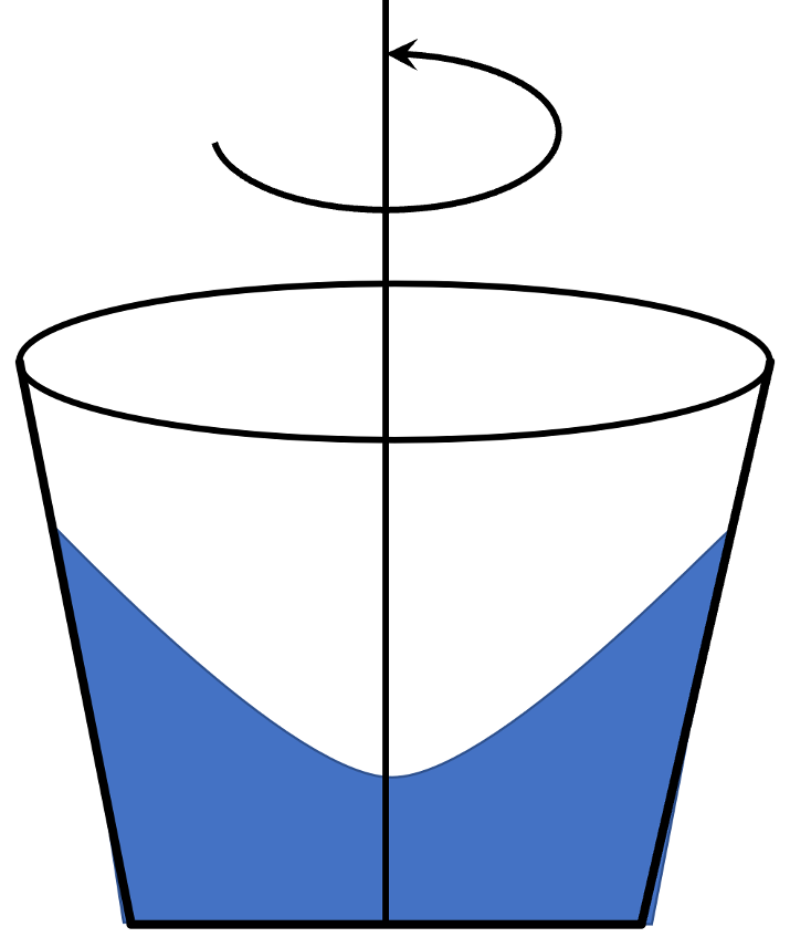
Now if we imagine that the bucket is then rotated about its vertical axis, our intuition says that the fluid will tend to migrate outwards leading to a parabolic-like profile that is lower at the center of the bucket and higher at the edges.
To mathematically prove our intuition, assume that the bucket spins uniformly so that its angular velocity is given by
\[ \vec \Omega = \left[ \begin{array}{c} 0 \\ 0 \\ \Omega \end{array} \right] \; \]
with the resulting fluid velocity being
\[ \vec V = \vec \Omega \times \vec r = \left[ \begin{array}{c} -\Omega y \\ \Omega x \\ 0 \end{array} \right] \; .\]
The fluid vorticity is
\[ \vec \omega = \nabla \times \vec V = \left[ \begin{array}{c} 0 \\ 0 \\ 2 \Omega \end{array} \right] \; .\]
Now we have two paths that we may try in incorporating these kinematic assumptions in the description of the free surface of the fluid: direct solution of Euler’s equation or application of Bernoulli’s theorem. The latter is certainly seems more attractive as it requires fewer steps but that it leads to a contradiction whose explanation proves to be informative. The direct solution is harder to implement but yields a solution consistent with our intuition. But, for the sake of pedagogy, let’s try Bernoulli’s theorem first.
The free surface of the fluid is defined by the locus of points in the fluid with a common pressure equal to atmospheric pressure. The fluid density is also assumed to be constant (a defining assumption of the ideal fluid theory we are using). Applying Bernoulli’s theorem, which reads
\[ \frac{P}{\rho} + g z + \frac{1}{2} \Omega \left( x^2 + y^2 \right) = C’ \; \]
to the entire fluid gives
\[ g z + \frac{1}{2} \Omega \left( x^2 + y^2 \right) = C \; .\]
Solving for z yields
\[ z = C – \frac{1}{2} \frac{\Omega^2}{g} \left( x^2 + y^2 \right) \; ,\]
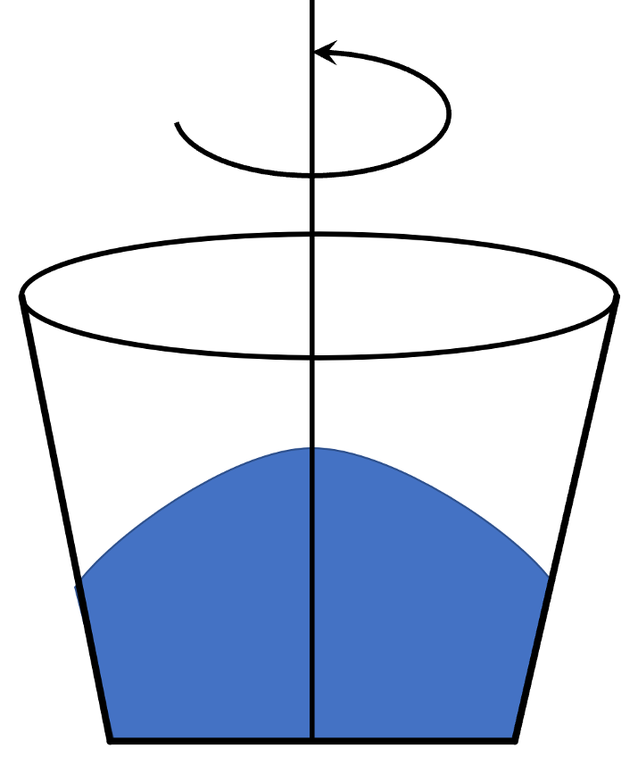
which is a free surface that is higher at the middle than it is at the edges, in clear contradiction to our experience and intuition.
So, what went wrong? The answer is that the flow is not irrotational (the vorticity presented above is not zero). The assumption that Bernoulli’s equation describes a quantity that is constant throughout the entire fluid doesn’t apply. The flow is steady, so $$(\vec V \cdot \nabla) H = 0$$ still holds, implying that $$H$$ is constant along a given streamline but there is no way to know how $$H$$ varies as we move from one fluid element to another. So, the blind application of Bernoulli’s theorem to every fluid element is simply not correct. Again this is a key reminder of the distinction between a quantity that stays constant along a streamline as the fluid flows and a quantity that is constant throughout every part of the fluid.
The correct way to solve this problem is to go back to Euler’s equation in component form. The make it a bit easier to apply, first compute some intermediate results. The nonlinear term in Euler’s equation becomes
\[ \left( \vec V \cdot \nabla \right) \vec V = \left( -\Omega y \partial_x + \Omega x \partial_y \right) \left[ \begin{array}{c} -\Omega y \\ \Omega x \\ 0 \end{array} \right] = \left[ \begin{array}{c} – \Omega^2 x \\ -\Omega^2 y \\ 0 \end{array} \right] \; . \]
The incompressibility relation
\[ \nabla \cdot \vec V = \partial_x (-\Omega y) + \partial_y (\Omega x) = 0 \; \]
is automatically satisfied so we can ignore it going forward.
Euler’s equation then becomes
\[ \left[ \begin{array}{c} -\Omega^2 x \\ -\Omega^2 y \\ 0 \end{array} \right] = -\frac{1}{\rho} \left[ \begin{array}{c} \partial_x P \\ \partial_y P \\ \partial_z P \end{array} \right] + \left[ \begin{array}{c} 0 \\ 0 \\ -g \end{array} \right] \; , \]
which, when simplified, becomes the three coupled partial differential equations
\[ \partial_x P = \rho \Omega^2 x \; , \]
\[ \partial_y P = \rho \Omega^2 y \; , \]
and
\[ \partial_x P = -\rho g \; . \]
Assuming the pressure to be a separable function of all three coordinates, we can integrate the first equation to get
\[ P = \frac{1}{2} \rho \Omega^2 x^2 + F(y,z) \; . \]
The second equation then becomes
\[ \partial_y P = \partial_y F(y,z) = \rho \Omega^2 y \; , \]
which results in
\[ F(y,z) = \frac{1}{2} \rho \Omega^2 y^2 + G(z) \; .\]
Finally, the third equation becomes
\[ \partial_z P = \partial_z G(z) = -\rho g \; , \]
which has the solution
\[ G(z) = -\rho g z \; ,\]
giving a final form of the pressure as
\[ P(x,y,z) = \frac{1}{2} \rho \Omega^2 x^2 + \frac{1}{2} \rho \Omega^2 y^2 – \rho g z \; .\]
Setting the pressure equal to the constant atmospheric pressure yields
\[ \frac{P_{atmosphere}}{\rho g} = const = \frac{1}{2} \frac{\Omega^2}{g} \left( x^2 + y^2 \right) – z \; \]
or
\[ z = \frac{1}{2} \frac{\Omega^2}{g} \left( x^2 + y^2 \right) – const \; ,\]
which is exactly the parabolic shape our intuition and common experience demands.
The lesson here is the vorticity is a key quantity that provides invaluable insight into fluid motion.