
Elementary Viscous Flow – Part 2
This month’s column finishes up the study of elementary viscous flow and presents the final two examples, both dealing with shear-induced flow. This type of flow (called Couette flow) typically results from the no-slip condition in which a moving boundary drags the fluid that touches it into motion. That layer of the fluid then drags the fluid layer next to it and so on.
For both of these examples, we are going to ignore body forces and external pressure differences and focus on the boundary motion alone. These assumptions eliminate several terms from the incompressible Navier-Stokes equations leaving us with
\[ \frac{\partial {\vec V}}{\partial t} + ( {\vec V} \cdot \nabla) {\vec V} = \nu \nabla^2 {\vec V} \; , \]
augmented with the usual incompressibility assumption $$\nabla \cdot {\vec V} = 0 $$.
Cylindrical Couette Flow
In this example, we imagine a fluid trapped between two cylindrical shells, an inner and an outer shell, of radii $$R_{inner} \equiv R_{1}$$ and $$R_{outer} \equiv R_{2}$$, respectively.
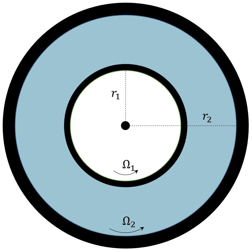
For sake of generality, both shells will be allowed to rotate about the vertical axis (out of the page) with angular velocities $$\Omega_{inner} \equiv \Omega_{1}$$ and $$\Omega_{outer} \equiv \Omega_{2}$$. We seek to describe the velocity profile of the fluid in steady motion. With the radii and angular velocities assumed to be known there will be a fairly simple relationship between the velocity profile and the kinematic viscosity $$\nu$$. A viscometer uses this experimental setup to measure kinematic viscosity by tracking the torque required to keep the inner shell moving at a constant rate (the out shell is usually fixed).
The Navier-Stokes equations are best presented in cylindrical coordinates since these coordinates match the geometry involved. The added benefit is that expressing the derivatives in cylindrical coordinates is instructive in its own right.
The key point to focus on is that in cylindrical coordinates, the basis vectors in directions perpendicular to the $$z$$-axis change as a function of azimuthal angle $$\theta$$. The radial unit vector changes as
\[ \partial_{\theta} {\hat e}_r = {\hat e}_{\theta} \; \]
and the azimuthal unit vector as
\[ \partial_{\theta} {\hat e}_{\theta} = – {\hat e}_r \; .\]
In steady flow, by symmetry, the velocity field is a function of radius alone
\[ {\vec V} = V_{\theta}(r) {\hat e}_{\theta} \; \].
The nabla operator takes the well-known form
\[ \nabla = \frac{1}{r} \partial_{r} ( r ) + \frac{1}{r} \partial_{\theta} + \partial_z \; .\]
Under the flow geometry assumptions, the convective portion of the material derivative becomes
\[ ({\vec V} \cdot \nabla) = \frac{V_{\theta}}{r} \partial_{\theta} \; .\]
Applying this operator to the velocity field yields
\[ ({\vec V} \cdot \nabla) {\vec V} = \left( \frac{V_{\theta}}{r} \partial_{\theta}\right) (V_{\theta} {\hat e}_{\theta}) = – \frac{V_{\theta}^2}{r} {\hat e}_{r} \; \]
The Laplacian of the vector field becomes
\[ \nabla^2 {\vec V} = \left( \partial_{r}^2 + \frac{1}{r} \partial_{r} + \frac{1}{r^2} \partial_{\theta}^2 \right) ( V_{\theta} {\hat e}_{\theta} ) = \left( \partial_{r}^2 V_{\theta}+ \frac{1}{r} \partial_{r} V_{\theta} – \frac{V_{\theta}}{r^2} \right) {\hat e}_{\theta} \; . \]
The assumption of steady flow then leaves the incompressible Navier-Stokes equations, in component form, as
\[ – \frac{V_{\theta}^2}{r} = \frac{1}{\rho} \partial_{r} P \; , \]
\[ 0 = – \frac{1}{\rho r} \partial_{\theta} P + \nu \left( \partial_{r}^2 V_{\theta} + \frac{1}{r} \partial_{r} V_{\theta} – \frac{V_{\theta}}{r} \right) \; , \]
\[ 0 = – \frac{1}{\rho} \partial_{z} P \; . \]
Note that the incompressibility condition is automatically satisfied by the form of the velocity field.
From the last equation the pressure cannot be a function of $$z$$ and since everything else in the second equation is only a function of $$r$$ so must $$\partial_{\theta} P = f(r)$$. Integrating gives
\[ P(r) = f(r) \theta + g(r) \; , \]
the form of which requires $$f(r) = 0$$ otherwise the pressure would be a multi-valued function. The second equation now becomes
\[ 0 = \nu \left( \partial_{r}^2 V_{\theta} + \frac{1}{r} \partial_{r} V_{\theta} – \frac{V_{\theta}}{r} \right) \; , \]
The general solution is
\[ V_{\theta} = A r + \frac{B}{r} \; .\]
In the interest of brevity, the solutions for the constants are
\[ A = \frac{ \Omega_{2} r_{2}^2 – \Omega_{1} r_{1}^2 }{r_{2}^2 – r_{1}^2} \; \]
and
\[ B = \frac{ (\Omega_{2} – \Omega{1}) r_{1}^2 r_{2}^2 }{ r_{2}^2 – r_{1}^2} \; , \]
which are easily obtained by applying the boundary conditions to the general relation $$V_{\theta} = r \Omega$$.
Once $$V_{\theta}$$ is known, the first equation gives the radial pressure gradient due to the rotation.
Linear Couette Flow
In this last example, we will solve the time varying Couette flow setup up between two plates separated by a distance $$w$$ and extending far in the $$x$$- and $$z$$-directions so that we can ignore the edge effects and model the flow as two-dimensional.
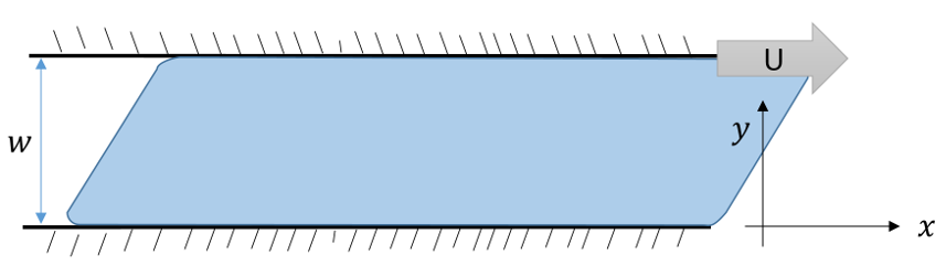 We imagine that the fluid is at rest prior to $$t=0$$ at which time the upper plate is set into motion with velocity $${\vec V} = U {\hat e}_x$$. There is a well-known steady solution in which the velocity linearly varies from zero on the lower plate to $$U$$ on the upper plate but it is interesting to see how the transient flow settles into this steady state.
By our earlier, assumptions, the flow is of the form (automatically satisfying the incompressibility condition)
\[ {\vec V} = V_x(t,y) {\hat e}_x \; , \]
which has to satisfy the following form of the Navier-Stokes equations
\[ \rho \partial_{t} V_x = \mu \partial_{y}^2 V_x \; . \]
The boundary conditions and initial condition are
\[ \textrm{BCs:} \;\;\;\;\;\;\;\; \left\{ \begin{array}{l} V_x(t,0) = 0 \\ V_x (t,w) = U \end{array} \right. \; \]
and
\[ \textrm{IC:} \;\;\;\;\;\;\;\; V_x(0,y) = 0 \;\;\;\;\; 0 \leq y \leq w \; , \]
respectively.
The solution strategy is to employ separation of variables. To that end, following Acheson, write the velocity as a sum of the steady solution and a time-varying piece where the latter has homogeneous boundary conditions
\[ V_x(t,y) = \frac{U}{w} y + {\tilde V}_x(t,y) = \frac{U}{w} y + f(t)g(y) \; . \]
After performing the separation of variables, we arrive at
\[ \frac{1}{\nu} \frac{1}{f} \partial_{t} f = – s_{n}^2 = \frac{1}{g} \partial_{y}^2 g \; , \]
where $$s_n$$ is a separation constant.
The spatial equation, $$g^{\prime\prime} + s_{n}^2 g = 0$$ has general solutions $$g(y) = A \sin (s_n y) + B \cos (s_n y) $$. Applying the boundary conditions requires $$B=0$$ and $$s_n = n \pi / w \;\; n = 1, 2, 3, \ldots$$. The time equation is easily integrated to $$f(t) = \exp( -s_n\nu t )$$. The general solution is
\[ V_x(t,y) = \frac{U}{w} y + \sum_{n=1}^{\infty} A_n \exp \left( – \frac{ n^2 \pi^2}{w^2} \nu t \right) \sin \left( \frac{n \pi}{w} y \right) \; . \]
The initial conditions are satisfied by picking the $$A_n$$ appropriately. The key to doing this is to exploit the orthogonality
\[ \int_0^w \sin \left( \frac{m \pi}{w} y \right) \sin \left( \frac{n \pi}{w} y \right) = \frac{w}{2} \delta_{mn} \; \]
to get
\[ A_m = -\frac{2}{w} \int_0^w \frac{Uy}{w} \sin \left( \frac{m \pi}{w} y \right) dy = \frac{ 2 U (-1)^n }{n \pi} \; . \]
The following plot shows this solution for $$w = 5mm$$ and $$\nu = 0.8926 mm^2/s$$.
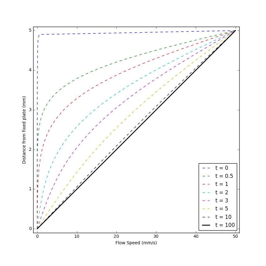
Note the majority of the velocity is confined near the top plate at short times (this is essentially the boundary layer) but how quickly the solution tends to the steady state.
As a way of seeing this boundary layer as a feature of the transient behavior consider what happens if the top plate moves in an oscillatory fashion with velocity $$U \cos (\omega t) $$. Assuming that the fluid velocity has the form $$ V_x(t,y) = f(y) e^{i \omega t} $$, the Navier-Stokes equations yield
\[ f” – i \omega/\nu f = 0 \; .\]
Following the usual strategy $$f = exp(\lambda y)$$ gives values
\[ \lambda_{\pm} = \pm e^{i \pi/4} \sqrt{\frac{\omega}{\nu}} \; .\]
Some spirited complex algebra leads to
\[ V_x(t,y) = U e^{-ky} e^{i (\omega t – k y) } \; ,\]
where $$k = \sqrt{\omega/2 \nu}$$. As the following animation shows, the velocity at the upper plate follows the motion of the plate but the main action is confined to a thin layer. Essentially, the motion is always transient and the influence of the fluid motion near the moving plate isn’t able to diffuse into the bulk of the fluid.