
Elementary Compressible Flow – Part 1
This month’s column briefly examines compressible fluid flow. This journey will be a short excursion into a rather complicated discipline with only two aims. The first is to give a flavor of how and why the energy equation, which has been essentially unused in previous analyses, plays a role and how additional thermodynamic information (spatial and temporal variations in density and temperature) comes into play. The second is to setup all the equations needed to understand the basic physics associated with that object that ushered in the space age: the rocket nozzle, which will be the subject of next month’s entry.
Following the usual introductory approaches (e.g. Eric R. Pardyjak’s online notes and Chapter 9 of Merle C. Potter’s Fluid Mechanics Demystified), we will look at only simplified geometries, such as the converging nozzle shown here
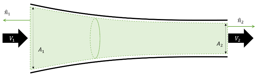
with a flow from left-to-right as indicated.
This analysis assumes that all of the flow variables are constant over each cross-section but can differ from cross-section to cross-section. The first condition means that the flow is effectively inviscid, since the boundary layer is ignorable for the vast majority of the flow, and it is steady. All of these simplifying assumptions result in algebraic flow equations that come from the integral forms of the fluid equations rather than the differential equations. In addition, we will ignore body forces (i.e. gravity) and only allow pressure-driven flows.
The conservation (i.e. Eulerian) form of the equations is slightly easier to work with and these will be our starting point for the various simplifications that we impose (although with one extra wrinkle in the case of energy). All of the derivations will involve some vector quantity (say the velocity $${\vec V}$$) being integrated over a surface after being projected onto the local surface normal. This process results in an average value of the normal component of the vector over the entire face. This quantity will be denoted simply as a scalar (e.g. $$V_1$$) with appropriate labeling indicating which segment of the bounding surface.
Continuity Equation
Our starting equation is
\[ \int_{{\mathcal Vol}} d {\mathcal Vol} \, \frac{\partial \rho}{\partial t} + \int_{{\mathcal S}} d {\mathcal S} \, \rho {\vec V} \cdot {\hat n} = 0 \; .\]
Since the flow is steady, the first term vanishes. If we imagine the surface as shown in the nozzle above, then only the flow through the endcaps ($${\mathcal S}_1$$ and $${\mathcal S}_2$$) is non-zero and
\[ \int_{{\mathcal Vol}} d {\mathcal Vol} \, {\vec V} = {\rho}_1 {\hat n}_1 \cdot {\vec V}_1 A_1 + {\rho}_2 {\hat n}_2 \cdot {\vec V}_2 A_2 = 0 \; .\]
Accounting for the direction of the flow relative to the respective normals we arrive at
\[ {\rho}_1 V_1 A_1 = {\rho}_2 V_2 A_2 \equiv {\dot m} \; . \]
Momentum Equation
Next, we consider the momentum equation expressed as
\[ \int_{{\mathcal Vol}} d {\mathcal Vol} \, \frac{\partial \left(\rho {\vec V}\right)}{\partial t} + \int_{{\mathcal S}} d {\mathcal S} \, (\rho {\vec V}) {\vec V} \cdot {\hat n} = \int_{{\mathcal S}} d {\mathcal S} \, {\mathbf T} \cdot {\hat n} \; ,\]
where $${\mathbf T}$$ is the Cauchy stress tensor. Following the same approach as above, and recalling that the body forces are zero (i.e. $${\mathbf T} = – P {\mathbf I}$$), the Cauchy momentum equation takes the form:
\[ {\rho}_1 {\vec V}_1 ( {\vec V}_1 \cdot {\hat n}_1) A_1 + {\rho}_2 {\vec V}_2 ( {\vec V}_2 \cdot {\hat n}_2) A_2 = -P_1 A_1 {\hat n}_1 – P_2 A_2 {\hat n}_2 \; .\]
Again taking into account the direction of the flow relative to the normals, we arrive at
\[ {\rho}_2 V_2 A_2 {\vec V}_2 – {\rho}_1 V_1 A_1 {\vec V}_1 = ( P_1 A_1 – P_2 A_2 ) {\hat n}_2 \; ,\]
where we’ve used $${\hat n}_1 = – {\hat n}_2$$. Two things are worth noting about this equation. First, the direction of the flow must be along (either parallel or anti-parallel) to the end-caps, nicely in keeping with the assumption that the flow varies only from cross-section to cross-section and not within a cross-section. Second, the continuity equation can be used to eliminate many of the terms in favor of the constant mass flow rate $${\dot m}$$. Keeping all this in mind brings us to the scalar equation
\[ {\dot m} (V_2 – V_1) = (P_1 A_1 – P_2 A_2) \; . \]
Energy Equation
Up to this point, we’ve not had to occasion to use the energy equation for the simple fact that in incompressible flows without explicit heat flows and generation, the internal energy of each fluid element remains constant; only the kinetic energy changed. Indeed, the energy equation for such a flow follows immediately by taking the dot product of the Cauchy momentum equation with the velocity. In these simple cases, the density is a given and only pressure and velocity are unknown. The four equations of continuity and 3 components of the Cauchy momentum equation sufficed to solve for the four unknowns.
Once we allow the flow to be compressible, the density becomes an unknown and the also the internal energy enters into the picture. The energy equation provides one more equation. The final equation comes from a thermodynamic equation of state. For this latter equation, we will assume the ideal gas law. Often, it is more convenient to switch from internal energy to temperature by using the ideal gas relation
\[ e = c_v T \]
and
Fourier’s law relating heat flow to temperature via
\[ {\vec q} = – k \nabla T \; .\]
There is an additional thermodynamic consideration (the one wrinkle mentioned at the beginning of this post). It is the introduction of the enthalpy $$h = e + P/\rho$$ that combines the internal energy with the pressure work. Its introduction is really a matter of convenience rather than an important insight but, as the majority of the discipline’s practioners uses it, it would be a mistake to omit.
To see how the energy equation admits its inclusion, start with the energy equation in its full glory
\[ \int_{{\mathcal Vol}} d {\mathcal Vol} \, \frac{\partial}{\partial t} \left[ \rho \left(e + \frac{V^2}{2} \right) \right] + \int_{{\mathcal S}} d {\mathcal S} \, \rho \left(e + \frac{V^2}{2} \right) {\vec V} \cdot {\hat n} = \\ \int_{{\mathcal Vol}} d {\mathcal Vol} \, \rho \left( {\vec a}_{body} \cdot {\vec V} + {\dot Q} \right) + \int_{{\mathcal S}} d {\mathcal S} \, \left( {\mathbf T} \cdot {\vec V} + {\vec q} \right) \cdot {\hat n} \; .\]
By the above assumptions, the volumetric heating and the heat flow are zero, the body forces are zero, the stress tensor simply accounts for the pressure, and the flow is steady. Under these conditions, the equation reduces to
\[ \int_{{\mathcal S}} d {\mathcal S} \, \rho \left(e + \frac{V^2}{2} \right) {\vec V} \cdot {\hat n} = – \int_{{\mathcal S}} d {\mathcal S} \, P {\vec V} \cdot {\hat n} \; .\]
Collecting terms gives
\[ \int_{{\mathcal S}} d {\mathcal S} \, \rho \left( e + \frac{P}{\rho} + \frac{V^2}{2} \right) {\vec V} \cdot {\hat n} = 0 \; , \]
or, when integrated, accounting for the normal on the endcaps, and using the definition of enthalpy
\[ \rho_2 V_2 A_2 \left( h_2 + \frac{{V_2}^2}{2} \right) – \rho_1 V_1 A_1 \left( h_1 + \frac{{V_1}^2}{2} \right)= 0 \; .\]
Summary
Finally, we can summarize all the relations
\[ \begin{array}{ll} {\textrm{continuity:}}& {\rho}_1 V_1 A_1 = {\rho}_2 V_2 A_2 \equiv {\dot m}\\{\textrm{momentum:}}& (\rho_1 V_1^2 + P_1) A_1 = (\rho_2 V_2^2 + P_2) A_2 \\{\textrm{energy:}}& h_1 + \frac{{V_1}^2}{2} = h_2 + \frac{{V_2}^2}{2} \end{array} \; , \]
which are basically the Rankine-Hugonoit jump conditions used in shock wave propagation analysis (assuming $$A_1 = A_2$$).
Next month we will apply these equations to elementary compressible fluid and the production of shocks.