
Elementary Compressible Flow – Part 4
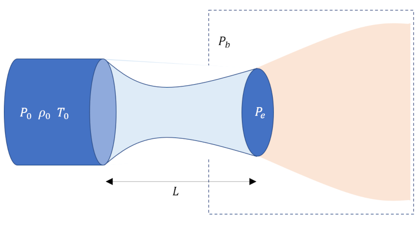
In this final post on compressible fluid flow, we will take a look at an application of the machinery developed over the previous three posts to the converging-diverging nozzle, often called a rocket nozzle or a de Laval nozzle. The setup in straightforward even though it is probably unfamiliar. We imagine a reservoir containing a gas at a high pressure and, not often, high temperature that serves to supply the flow through the nozzle. By convention, the thermodynamic state variables in the reservoir are given a ‘0’ subscript and are called the stagnant conditions as there is no flow within the reservoir itself. This reservoir feeds into a converging section of a nozzle in which the cross-sectional area decreases steadily until a minimum occurs at what is called the throat of the nozzle. After the throat, the cross-sectional area increases again until the nozzle ends at the exit. The nozzle and reservoir are placed into a larger pressure vessel (sometimes called the receiver) where the pressure outside of the exit, called by convention the back pressure, $P_b$.
Initially the two pressures are equal and there is no flow from the reservoir through the nozzle. As the back pressure is dropped, flow develops from the reservoir. de Laval’s innovation was to realize that if the flow can be brought to sonic conditions (i.e., Mach number $M=1$) at the throat then the diverging section would further speed up the flow to supersonic speeds (see the discussion at the end of the second post of this series).
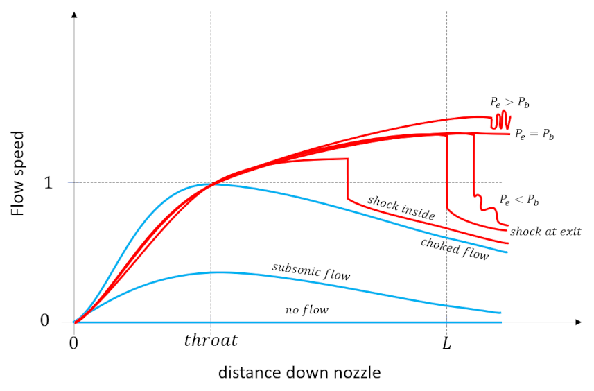
The goal of this post is to discuss the flow profiles along the length of the nozzle, from inlet at the reservoir, to exit into the pressure vessel, as a function of the ratio $P_b/P_0$ and to give a flavor of how the previous equations are used to quantitatively. Despite the relative simplicity of the system (reservoir, nozzle, and pressure vessel) a rich set of flow patterns result. Qualitatively, these fall into two broad classes with several variations within them.
In the first class (shown in blue traces in the figure below), the flow is everywhere isentropic from the reservoir. through the nozzle, and into the pressure vessel. Included in this class is the flat trace where $P_b/P_0 = 1$ where no flow results. As $P_b/P_0$ is lowered, flow commences with the speed of the flow increasing as it approaches the throat from the converging section and then subsequently slowing down in the diverging section. The maximum speed in the nozzle (which for this class is always at the throat) continues to increase until as $P_b/P_0$ is lowered until a critical value of the back pressure, $P_{b_s}$ when the flow is sonic (i.e., $M=1$) in the throat but still subsonic everywhere else in the nozzle (including the diverging section).
At this point, lowering the $P_b/P_0$ ratio further develops the second class of flow (shown in red traces in the figure below) where some portion of the flow in the diverging section is supersonic. A shock develops somewhere downstream of the throat in order to decelerate the flow back to subsonic conditions so that it can match boundary conditions with the environment in the pressure vessel. The only remaining question is precisely where the shock is found. Five possible options are available: 1) the shock is found in the nozzle between the throat and the exit, 2) the shock falls at the exit, 3) the shock is beyond the nozzle but the exit pressure $P_e < P_b$, 4) the shock is beyond the nozzle and $P_e = P_b$, and 5) the shock is beyond the nozzle but $P_e > P_b$. Options 3), 4), and 5) are called over-expanded, perfectly-expanded, and under-expanded flows, respectively (see discussion of The Converging-Diverging Nozzle applet).
In the third post of this series, we derived expressions relating the pressure, density, and temperature anywhere in an isentropic portion of the flow to the stagnation properties in the reservoir. The relations derived were:
\[ \frac{P_0}{P} = \left[1 + \frac{\gamma – 1}{2} M^2 \right]^{\frac{\gamma}{\gamma -1}} \; ,\]
\[ \frac{\rho_0}{\rho} = \left[1 + \frac{\gamma – 1}{2} M^2 \right]^{\frac{1}{\gamma -1}} \; ,\]
and
\[ \frac{T_0}{T} = 1 + \frac{\gamma – 1}{2} M^2 \; .\]
We also derived the area-Mach number relationship, (AMR),
\[ \frac{A}{A^*} = \frac{1}{M} \left(1 + \frac{\gamma – 1}{2} \right)^{\frac{\gamma+1}{2(1-\gamma)}} \left[ 1 + \frac{\gamma – 1}{2} M^2 \right]^{\frac{\gamma+1}{2(\gamma-1)}} \; \]
that specified what the ratio of the local area, $A$, to the area of the throat, $A^*$, must be to achieve a target value of Mach number $M$. A typical problem where these equations are useful comes from Fluid Mechanics Demystified by Merle Potter and reads
Air flows through a converging-diverging nozzle attached to a reservoir maintained at 400 kPa absolute and 20$^{\circ}$C to a receiver. If the throat and exit diameters are 10 and 24 cm, respectively, what is the receiver pressure that will just result in supersonic flow throughout the diverging portion of the nozzle.
The solution starts with recognizing that if the flow in the diverging portion of the nozzle is to be supersonic then choked conditions occurs at the throat and, as a result, the throat area coincides with the critical area $A_{throat} = A^*$. The area ratio of the exit to the throat is then $\frac{A}{A^*} = \left( \frac{24}{10} \right)^2=5.76$. Next we have to invert the AMR to find the value of $M$ that corresponds to this ratio. A bisection, specifically adapted to the two possible dynamical behaviors: subsonic and supersonic, was written in python. The resulting value was $M=3.3244$ was then plugged into the $P_0/P$ relation and the reciprocal taken to arrive at the exit pressure being $P_{exit} = 6746.659 \, Pa$, corresponding to an exit pressure only about $1.6%$ as large as the stagnant pressure.
The possibility of a shock in the possible flows requires us to add three new relations to our collection. Our starting point for deriving the so-called jump conditions across the shock are the three basic fluid equations for mass, momentum, and energy, derived in the first post, but simplified by the tacit assumption that the shock is negligibly thick so that the cross-sectional area is the same on both sides of the shock, giving:
\[ \rho_u V_u = \rho_d V_d \; , \]
\[ (\rho_u {V_u}^2 + P_u) = (\rho_d {V_d}^2 + P_d) \; ,\]
and
\[ h_u + \frac{{V_u}^2}{2} = h_0 = h_d + \frac{{V_d}^2}{2} \; , \]
respectively. Note that the subscripts `u’ and `d’ stand for upstream and downstream, respectively.
As before, our thermodynamics will assume the fluid to be an ideal gas with the equation of state given by $P/\rho = R T$. The general form of enthalpy $h = e + P/\rho$ takes the simple form $h = (\gamma/\gamma-1) P/\rho$. The state variables relate to their values at different parts of the flow via
\[ \frac{P_0}{P} = \left( \frac{\rho_0}{\rho} \right)^{\gamma} = \left( \frac{h_0}{h} \right)^{\frac{\gamma}{\gamma-1}} \; . \]
The speed of sound in the gas, which is temperature dependent, takes on the forms
\[ c = \sqrt{\gamma R T } = \sqrt{\frac{\gamma P}{\rho}} = \sqrt{(\gamma-1) h} \; , \]
each useful in context.
Finally, the energy equation, which had been relegated to a by-stander role in incompressible fluid flow, offers two very useful relations. The first, which will be termed the stagnant enthalpy expression (SEE), expresses the stagnant enthalpy in terms of the local sound speed via $(\gamma -1) h = c^2$ giving
\[ h_0 = h + \frac{V^2}{2} = h \left(1 + \frac{V^2}{2h} \right) = \frac{c^2}{\gamma-1} \left(1 + \frac{\gamma – 1}{2} M^2 \right) \; . \]
The second, which will be termed the local enthalpy expression (LEE), expresses the local enthalpy in terms of the local flow speed by
\[ (\gamma – 1) h = (\gamma – 1) \left( h_0 – \frac{1}{2}V^2 \right) \; . \]
One caution when using these relations. The reservoir is operational defined as the location where the flow is isentropically brought to a stop. Since a shock produces a great deal of entropy for any fluid element crossing from one side to another, the downstream thermodynamic conditions for a reservoir will be different from the actual reservoir attached to the nozzle and care must be taken not to confuse the notional one with the actual physical one.
To derive the normal shock relations, we follow these notes.
Begin by dividing the momentum equation by the mass continuity equation to get
\[ V_u – V_d = \frac{1}{\gamma} \left( \frac{{c_d}^2}{V_d} – \frac{{c_u}^2}{V_u} \right) \; . \]
Eliminate the local speeds of sound by relating them to their local enthalpies and then using the LEE to get
\[ V_u – V_d = \frac{\gamma -1}{\gamma} \left[ \frac{h_0 (V_u – V_d)}{V_u V_d} + \frac{1}{2}(V_u – V_d) \right] \; .\]
Dividing both sides by $V_u – V_d$ and rearranging yields
\[ \left( \frac{\gamma+1}{2} \right)^2 = \frac{h_0^2 (\gamma-1)^2}{{V_u}^2 {V_d}^2 } \; .\]
Next, employ a neat trick by writing the numerator on the left-hand side as ${h_0}^2 (\gamma-1)^2 = h_{0u} (\gamma-1) h_{0d} (\gamma – 1) $. Use the SEE to express each of these expressions in terms of the local sound speed and Mach number. Doing so yields
\[ \left( \frac{\gamma+1}{2} \right)^2 = \frac{1}{{M_u}^2} \left[1 + \frac{\gamma-1}{2} {M_u}^2 \right] \frac{1}{{M_d}^2} \left[1 + \frac{\gamma-1}{2} {M_d}^2 \right] \; . \]
Solving for $M_d$ is relatively painless with the substitutions $L = (\gamma-1)/2$ and $Q = (\gamma +1)/2$. These auxiliary variables keep the clutter down and the observation that $L^2 – Q^2 = -\gamma$ simplifies things enormously so that we arrive at
\[ {M_d}^2 = \frac{1 + \left(\frac{\gamma – 1}{2}\right) {M_u}^2 }{\gamma {M_u}^2 – \left( \frac{1-\gamma}{2} \right)} \; . \]
This relation allows u get the jump in all of the local thermodynamic variables. Starting with the density, use the continuity equation to
\[ \frac{\rho_d}{\rho_u} = \frac{V_u}{V_d} = \frac{{V_u}^2}{V_u V_d} \; .\]
Using the definition of Mach number and the SEE together yields
\[ {V_u}^2 = \frac{(\gamma-1)h_0}{1 + \frac{\gamma-1}{2} {M_u}^2} {M_u}^2 \; . \]
Earlier in the derivation of the Mach jump relations we found that $1/V_u V_d = (\gamma+1)/2 h_0(\gamma-1)$. Substituting these expressions back into the density equation yields
\[ \frac{\rho_d}{\rho_u} = \frac{(\gamma+1) {M_u}^2}{2 + (\gamma-1){M_u}^2} \; . \]
The momentum equation gives
\[ P_d – P_u = \rho_u {V_u}^2 – \rho_d {V_d}^2 = \rho_u {V_u}^2 \left(1 – \frac{\rho_d V_d V_d}{\rho_u V_u V_u} \right) = \rho_u {V_u}^2 \left(1 – \frac{\rho_u}{\rho_d} \right)\; . \]
Substitute $\rho V^2 = \gamma P M^2$ from the definition of the speed of sound and dividing by $P_u$ gives
\[ \frac{P_d}{P_u} – 1 = \gamma {M_u}^2 \left( 1- \frac{\rho_u}{\rho_d} \right) \; . \]
Using the already obtained expression for the density ratio (and noting to flip it based on which density is in the numerator) followed with some simplifications gives
\[ \frac{P_d}{P_u} = 1 + \frac{2\gamma}{\gamma+1} \left( {M_u}^2 – 1 \right) \; . \]
Finally, when needed, the temperature ratio comes subtituting into the ideal gas equation of state the ratios for density and pressure
\[ \frac{T_d}{T_u} = \frac{P_d}{P_u} \frac{\rho_u}{\rho_d} = \left[ 1 + \frac{2\gamma}{\gamma+1} \left( {M_u}^2 – 1 \right) \right] \frac{2 + (\gamma-1){M_u}^2}{(\gamma+1) {M_u}^2} \; .\]
We are now in a position to solve another typical problem associated with converging-diverging nozzle design, again taken from Merle Potter, that reads
Air flows from a reservoir through a nozzle into a receiver. The reservoir is maintained at $400 kPa$ absolute and $20{}^\circ C$. The nozzle has a 10-cm-diameter throat and a 20-cm-diameter exit. What is the back pressure that locates the shock wave at the exit?
Since the shock is at the exit, we can assume that the upstream side of the shock is supersonic at the area of the exit. So, the value of $A/A* = 4$. Using the inverse AMR function, the upstream Mach number is $M_u = 2.940$. Then using the standard isentropic relations the pressure ratio is $P_u/P_0 = 0.0298$ resulting in an upstream pressure of $P_u = 11,914.79 Pa$. Finally, the Mach shock jump relationship yields $P_d/P_u = 9.919$ for a downstream pressure, which is equal to the receiver pressure, of $P_d = 118179.93 Pa$.
Of course, this analysis just barely scratches the surface but these basic relations demonstrate the interplay between three basic laws of fluid mechanics: continuity, momentum, and energy and how they contribute to the practical construction of a converging-diverging nozzle. And, so, I guess this is rocket science.