
Thermodynamic Partials – Maxwell’s Relation
Last month’s installment presented a clean derivation of the classic relations between partial derivatives and showed a simple example of how they work in the concrete. As nice as that presentation is, the real power of these relations is only realized when dealing with systems with a large number of variables in play and in which various manipulations are required to extract meaning from the systems involved. The prototypical example is classical thermodynamics.
The fundamental concept in thermodynamics is the existence of a thermodynamic potential, which is a scalar function that encodes the state of the thermodynamic system in terms of the measurable quantities that describe the system, such as volume or temperature. Changes in the values, these independent physical variables (sometimes called the natural variables), relate directly to the potential of the corresponding partial derivatives.
The textbook example of this type of relation is defined in the first law of thermodynamics, which asserts that there exists a function, called the internal energy $$U$$, that is a function of the entropy $$S$$, the volume $$V$$, and the number of particles $$N$$ making up the physical system being modeled (assuming a single type of substance; generalizations to multiple species is straightforward but cumbersome). Changes in the internal energy $$U$$ can be calculated by
\[ dU = T dS – P dV + \mu dN \; ,\]
where the temperature, pressure and chemical potential are defined as
\[ {T} = \left( \frac{\partial U}{\partial S} \right)_{V,N} \; , \]
\[ {P} = -\left( \frac{\partial U}{\partial V} \right)_{S,N} \; , \]
and
\[ {\mu} = \left( \frac{\partial U}{\partial N} \right)_{S,V} \; , \]
respectively.
Without dwelling on the theory, suffice it to stay that laboratory conditions vary and there are many circumstances where it is preferable to work with a different set of independent variables. For example, heating water on a stove top in an uncovered pan is better understood in terms of fixed pressure rather than fixed volume.
Thermodynamics supplies an approach for dealing with these cases using the Legendre transformation. In the stove-top experiment mentioned above, the appropriate potential is called the enthalpy, defined as
\[ H = U + PV \; . \]
Taking the first differential gives
\[ dH = dU + P dV + V dP \\ = T dS – P dV + \mu dN + P dV + V dP \\ = T dS + V dP + \mu dN \; , \]
which demonstrates that $$H = H(S,V,N)$$.
Assuming that the order of differentiation can be exchanged, there are several relationships that exist (called Maxwell relations) between various partial derivatives. For example:
\[ \left( \frac{\partial T}{\partial V} \right)_{S,N} = \left( \frac{\partial }{\partial V } \left( \frac{\partial U}{\partial S} \right)_{V,N} \right)_{S,N} \\ = \left( \frac{\partial }{\partial S} \left( \frac{\partial U}{\partial V} \right)_{S,N} \right)_{V,N} \\ = -\left( \frac{\partial P}{\partial S} \right)_{V,N} \; . \]
Obviously, there is a lot of notational overhead in the above relation. For the sake of this analysis, we will make two simplifications to improve the clarity. First, we will assume a single species with a fixed number of moles. This assumption removes the need to carry $$N$$ and $$\mu$$. Second, we will forego keeping track of the other variables being held constant. Since we will be tacitly tracking which thermodynamic potential is being used, there is little chance of confusion.
The primary purpose the Maxwell relations serve is to eliminate terms involving the entropy in favor of physical parameters that can be experimentally measured, such as temperature, volume, or pressure.
A useful mnemonic exists for looking up the various relations without scanning through a table. It’s called the thermodynamic square, and it’s constructed as below
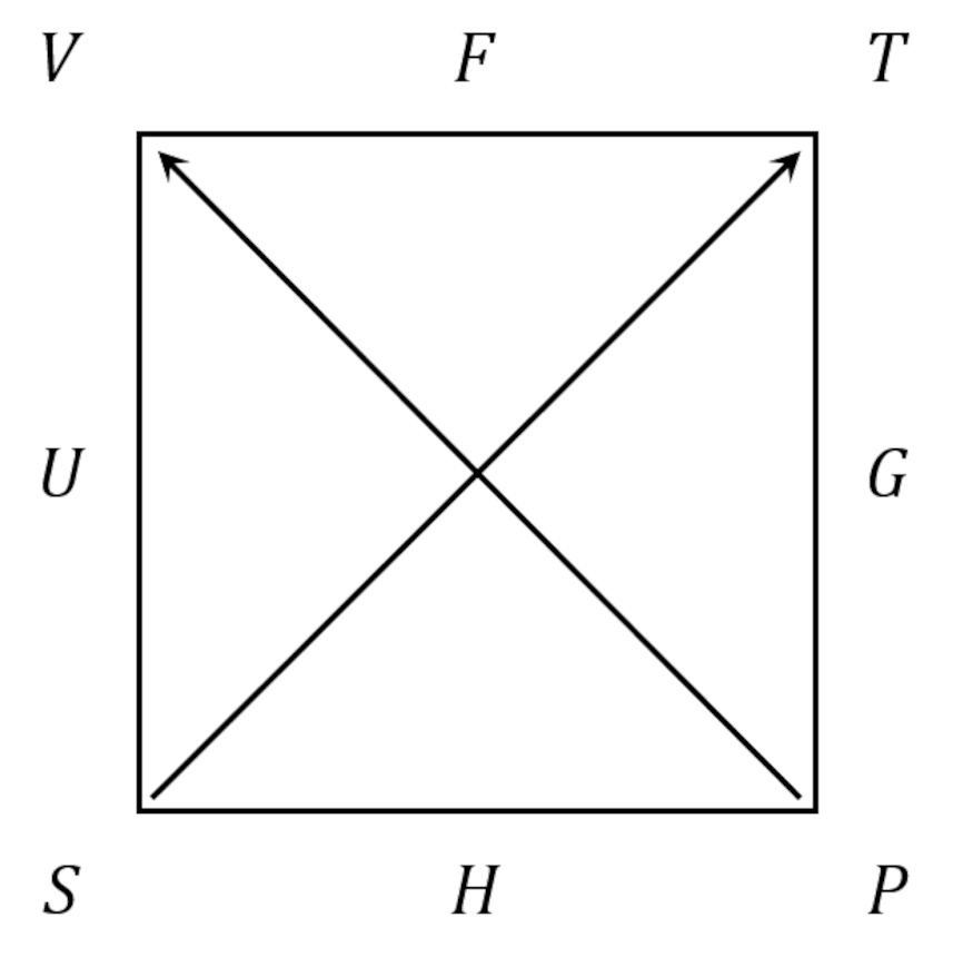
The 4 most important thermodynamic potentials, the Helmholtz free energy $$F = U – TS$$, the Gibbs free energy $$G = U + PV – TS$$, the enthalpy $$H = U + PV$$, and the internal energy $$U$$, are arranged along the edges starting up at the top and going clockwise. The thermodynamic variables – the temperature $$T$$, the pressure $$P$$, the entropy $$S$$, and the volume $$V$$ – are arranged at the corners, starting just after $$F$$ and also going clockwise. The Maxwell relations relate a partial derivative expressed in terms of three consecutive corners (shaded blue below) to the partial derivative expressed in terms another three consecutive corners (shaded yellow). The arrows lying along the diagonal set the sign of the partial derivative based on which variable is in the numerator: those with the arrowhead positive and those without negative.
These rules are far easier to understand with the mixed partial derivatives of $$U$$ discussed above.
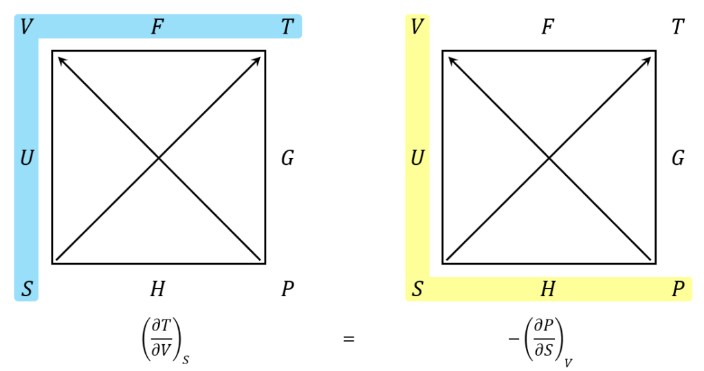
The blue shaded region reads counterclockwise while the yellow region reads clockwise. These orientations follow from the overlap they share on the left-hand side of the square (the one labeled $$U$$). The signs are determined by the arrows. Since the $$T$$ corner is the numerator and it has an arrowhead, the partial derivative is positive. Likewise, since the $$P$$ corner is the numerator and it lacks an arrowhead, the partial derivative is negative.
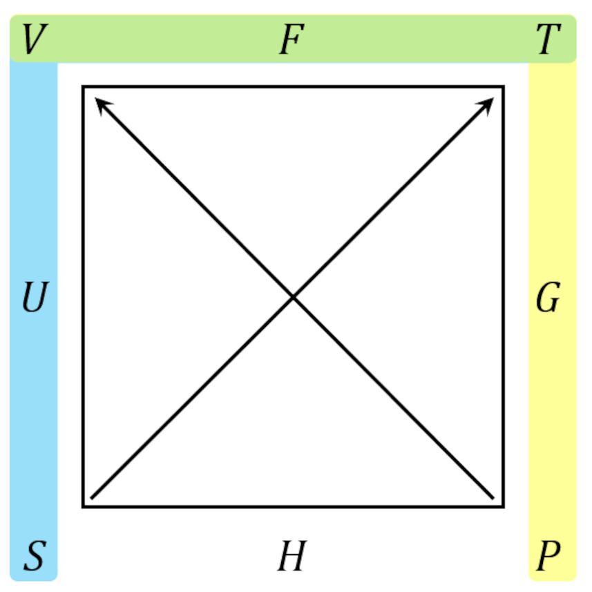
Once the basic operations using the square are understood, it is easier to present a single square with the common side being both shaded in blue and yellow, resulting in green. An example for the Maxwell relations coming from the Helmholtz free energy $$F$$ being
With these tools, we can get to the meatier topics, namely using a combination of the classical rules for partial derivatives and the Maxwell relations, as presented in the thermodynamic square, to eliminate the entropy in favor of physically measurable quantities. But this will be the topic for next month’s post.