
A Binomial Gas
The last installment discussed Robert Swendsen’s critique of the common, and in his analysis, erroneous method of understanding the entropy of a classical gas of distinguishable particles. As discussed in that post, his aim in making this analysis is to persuade the physics community to re-examine its understanding of entropy and to rediscover Boltzmann’s fundamental definition based on probability and not on phase space volume. To quote some of Swendsen closing words:
On the question of how this special case blossomed into textbook dogma we will have to content ourselves with speculations. It seems likely that the passion by which quantum mechanics gripped the physics community made it attractive to view the entire world through the lens of indistinguishable particles. Furthermore, quantum mechanics also elevated the concept of phase space since various dimensions could be viewed as canonically conjugate variables subject to the uncertainty principle. So, it is plausible that the physics community, dazzled by this new theory of the subatomic, latched onto the special case and ignored Boltzmann’s fundamental definition. If true, this would be incredibly ironic since the key focus of Boltzmann was on probability which is arguably the most shocking and intriguing aspect of quantum mechanics.
Regardless of these finer points of physics history, since the concept of probability is key in deriving the correct formula for a classical distinguishable gas let’s focus on the toy example Swendsen provides in order to illustrate his point. As in the last post, we will assume that the average energy per particle $
If we imagine a system with $N$ total distinguishable particles distributed between a volume $V$ partitioned into sub-volumes $V_1$ and $V_2$ then the probability $P(N_1,N_2)$ of having $N_1$ particles in $V_1$ and $N_2 = N – N_1$ in $V_2 = V – V_1$ is given by the binomial distribution
\[ P(N_1,N_2) = \left( \begin{array}{c} N \\ N_1 \end{array} \right) p^{N_1} (1-p)^{N_2} \; ,\]
where $p$ is the probability of being found in $V_1$ (i.e. a ‘success’). Since there are no constraints forcing particles to accumulate in any one section compared to the others they will distribute randomly within the entire domain. Therefore, $p = V_1/V$ and the probability is given by
\[ P(N_1,N_2) = \left( \frac{N!}{N_1! N_2!} \right) \left( \frac{V_1}{V} \right)^{N_1} \left( \frac{V_2}{V} \right)^{N_2} \; .\]
This expression is Swendsen’s launching point for deriving the correct expression for a classical gas of distinguishable particles. But before continuing with the analysis it is worth taking a few moments to better understand the physical content of that expression (even for those you understand the binomial distribution well).
There is a very compact way to make a Monte Carlo simulation of this thought experiment using the python ecosystem. One starts by defining a random realization of the classical gas particles placed within the volume and then reporting out the macroscopic thermodynamic state.
def particles_in_a_box(V1,N,V):
    import numpy as np

    #get random positions of the particles
    pos = np.random.random(N)

    #count number in subvolume V1
    threshold = V1/V
    return len(np.where(pos<threshold)[0])
In this context, the macroscopic thermodynamic state is a measure of how many particles are found in the sub-volume $V_1$. This is a critical point, particularly in light of the quantum interpretation that so many have embraced: two thermodynamic states can be identical without the underlying microstates being the same. For example, if $N=3$ and $N_1=2$ then each of the following lists results in the same thermodynamic state:
- [True,True,False]
- [True,False,True]
- [False,True,True]
where True and False result from the call to the numpy.where function and indicate whether the particle is found within $V_1$ (True) or not (False).
To get the probabilities, one makes an ensemble of such systems and this is what the following function does
def generate_MC_estimate(V1,N,V,num_trials):
    import numpy as np
    results = np.zeros(num_trials)
    for i in range(num_trials):
        results[i] = particles_in_a_box(V1,N,V)
    return results
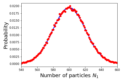
The following plot shows how well the empirical results for an ensemble with 100,000 realizations agree with the formula derived above for a simulation of 2000 particles placed in a box where $V_1 = 0.3 V$.
Following Boltzmann, the entropy is
\[ S = k \ln P + C = k \ln \left[ \left( \frac{N!}{V^{N_1}V^{N_2}}\right) \left( \frac{{V_1}^{N_1}}{N_1 !} \right) \left( \frac{{V_2}^{N_2}}{N_2 !} \right) + C \right] \; ,\]
where the previous expression has been grouped into parts dealing with the entire subsystem $(N,V)$, the first sub-volume $(N_1,V_1)$, and the second subsystem $(N_2,V_2)$. The constant $C$ depends only the whole system $N$ and $V$ but not on the subdivisions and, for reasons that should become obvious, we will take it to be
\[ C = – k \ln \left( \frac{{V}^{N}}{N !} \right) \; . \]
We first expand the entropy expression along this grouping to get
\[ S = k \ln \left( \frac{N!}{{V}^{N}} \right) + k \ln \left( \frac{{V_1}^{N_1}}{N_1 !} \right) + k \ln \left( \frac{{V_2}^{N_2}}{N_2 !} \right) – k \ln \left( \frac{{V}^{N}}{N !} \right) \; .\]
The first and last terms are inverses of each other and, under the action of the logarithm, cancel, leaving
\[ S = k \ln \left( \frac{{V_1}^{N_1}}{N_1 !} \right) + k \ln \left( \frac{{V_2}^{N_2}}{N_2 !} \right) \; .\]
As the whole is a sum of the parts, this expression is clearly extensive.
The final step is the application of Sterlings approximation ($\ln n! \approx n \ln n – n$). To keep things clear, we will apply it to terms of the form
\[ S = k \ln \left( \frac{V^N}{N!} \right) \; \]
to get
\[ S = k \left( \ln V^N – \ln N! \right) = k \left( N \ln V – N \ln N – N \right) = k N \left( \ln \frac{V}{N} – 1 \right) \; , \]
which clearly shows that $S$ scales linearly with the system size (at least in the thermodynamic limit).
All told, Swendsen argues persuasively that the correct interpretation of the entropy is that it is always proportional to the logarithm of the probability, that the ‘traditional’ expression depending on the volume of phase is a special case of the larger rule, and that by misapplying this special case large numbers of physicists have taught or have been taught incorrectly for decades. So much for the ideas of settled science.