
Enter Entropy
Up to this point in this classical survey of entropy, the star player, namely entropy itself has remained unseen but perhaps felt or anticipated. In this post, we actually get to the definition of entropy from the phenomenological point of view that is equilibrium thermodynamics.
To recap, we’ve covered the following points. To begin, the first law of thermodynamics neither restricts the types of allowed energy transformations nor the direction, order, or frequency. Like a good accountant working with double entry bookkeeping, the first law merely insists that the books balance and that energy losses from one account are balanced with gains in others – in short that energy is conserved. Next, we have the postulates of Clausius and Kelvin, which, much like financial regulators, place (or at least assert that nature places) restrictions on the types of allowed transactions. These restrictions naturally led to the notion of energy transfers falling into two broad categories: reversable and irreversible. Third, we find that the Carnot engine, with is incredibly simple set of 4 reversible processes, provides profoundly universal conclusions including the facts that the Kelvin and Clausius postulates each logically imply the other and that both are just two of many different facets of the larger second law of thermodynamics (although we stopped short of stating this in no uncertain terms since we hadn’t yet defined classical entropy). Finally, we established that no engine in the world can match the efficiency of the Carnot engine which is given by
\[ \epsilon_{Carnot} = 1 – \frac{|Q_H|}{|Q_L|} \; , \]
where $|Q_H|$ and $|Q_L|$ are the amounts of heat extracted from and dumped to the high ($T_H$) and low ($T_L$) temperature reservoirs, respectively. This implies that irreversibility is tied to the limitations found within the second law but this expression is hard to use since the amount of heat moved into or out during the cycle depends on the nature of the working substance.
To see this connection more clearly, let’s return to the Carnot engine but this time specifying the working substance to be an ideal gas with the familiar equation of state
\[ P V = n R T \; , \]
which we will use on each leg of the Carnot cycle, shown below.
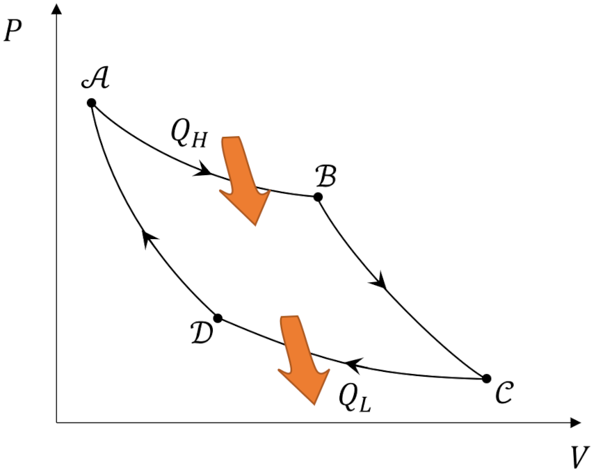
As a reminder, we are using the Clausius sign convention that assigns positive values to heat that flows into the ideal gas (system for short) and to work done by the system on its surroundings so that the first law reads $\Delta U = Q – W$. The pair of points ${\mathcal A}$ and ${\mathcal B}$ and the pair ${\mathcal C}$ and ${\mathcal D}$ are connected by isotherms. We’ll take, as given, the well-known result that the internal energy of an ideal gas depends only on temperature so along these isotherms $\Delta U_{{\mathcal A} \rightarrow {\mathcal B}} = 0 $ and $\Delta U_{{\mathcal C} \rightarrow {\mathcal D}} = 0$. From the first law, the constancy of the internal energy means that the heat that enters or exits the system is identically equal to the work: $Q_H = -W_{{\mathcal A} \rightarrow {\mathcal B}}$ and $Q_L = -W_{{\mathcal C} \rightarrow {\mathcal D}}$. Each of these works can be calculated easily by relating the pressure work $dW = P dV$ to the equation of state.
For the isothermal expansion
\[ Q_H = -W_{{\mathcal A} \rightarrow {\mathcal B}} = \int_{{\mathcal A}}^{{\mathcal B}} P d V \; .\]
Solving the equation of state for the pressure, substituting that result into the integral to eliminate $P$ and pulling out the constant temperature $T_H$ gives
\[ Q_H = n R T_H \int_{{\mathcal A}}^{{\mathcal B}} \frac{d V}{V} = n R T_H \ln \left( \frac{V_{{\mathcal B}}}{ V_{{\mathcal A}}}\right)\; .\]
As a check, note that since $V_{{\mathcal B}} > V_{{\mathcal A}}$ the heat transferred between the system and the higher temperature reservoir is positive ($Q_H > 0$) and that the work is negative ($W < 0$) since the system ‘pushes on’ the surrounding as it expands, both of which are consistent with the Clausius sign convention.
A similar analysis for the isothermal compression gives
\[ Q_L = n R T_L \ln \left( \frac{V_{{\mathcal D}}}{ V_{{\mathcal C}}}\right)\; .\]
As additional check, note that since $V_{{\mathcal D}} < V_{{\mathcal C}}$, that the heat transferred between the system and the lower temperature reservoir is negative ($Q_L$) representing heat flowing out, as expected.
We can now eliminate the volumes at each end state from these expressions for the heat flows by relating $T$ and $V$ on the adibats. The heat flow, by definition, is zero on these processes meaning that $\delta U = – W$. We will also assume that the ideal gas is calorically perfect so that the heat capacity at constant volume $C_V$ is a constant so that internal energy, which only depends on temperature, can be expressed as
\[ d U = n C_V d T \; . \]
Setting this expression equal to the work $dW = – P dV$ and eliminating the pressure using the equation of state gives
\[ C_V dT = -\frac{R T}{V} dV \; , \]
which can be immediately integrated from initial to final values to give
\[ \frac{T_f}{T_i} = \left( \frac{V_f}{V_i}\right)^{-\frac{R}{C_V}} = \left( \frac{V_f}{V_i}\right)^{1- \gamma}\; , \]
where the ratio $R/C_V$ is replaced with $\gamma – 1$ to match the usual convention. Finally, cross-multiplication to gather initial and final values on the left- and right-hand sides, respectively, yields
\[ T_i V_i^{\gamma – 1} = T_f V_f^{\gamma – 1} \;. \]
Applying this formula to the adiabatic expansion from ${\mathcal B} \rightarrow {\mathcal C}$ and the adiabatic compression from ${\mathcal D} \rightarrow {\mathcal A}$ gives
\[ T_H V_{{\mathcal B}}^{\gamma – 1} = T_L V_{{\mathcal C}}^{\gamma – 1} \; \]
and
\[ T_H V_{{\mathcal A}}^{\gamma – 1} = T_L V_{{\mathcal D}}^{\gamma – 1} \; .\]
Dividing the previous equation by the last one gives
\[ \frac{ T_H V_{{\mathcal B}}^{\gamma – 1}}{ T_H V_{{\mathcal A}}^{\gamma – 1}} = \frac{ T_L V_{{\mathcal C}}^{\gamma – 1}}{ T_L V_{{\mathcal D}}^{\gamma – 1}} \; ,\]
which simplifies to
\[ \frac{V_{{\mathcal B}}}{V_{{\mathcal A}}} = \frac{ V_{{\mathcal C}}}{ V_{{\mathcal D}}} \; .\]
These ratios enable us to eliminate the volumes from the computations of heat obtained from analyzing the isothermal steps leaving us with
\[ \frac{Q_H}{T_H} = \frac{-Q_L}{T_L} \; ,\]
where ‘extra’ minus sign come from flipping $V_{{\mathcal D}}/V_{{\mathcal C}}$ in the original expression to $V_{{\mathcal C}}/V_{{\mathcal D}}$. The question of sign convention can be totally eliminated by with absolute values to
\[ \frac{|Q_H|}{T_H} = \frac{|Q_L|}{T_L} \; .\]
The simplicity of this expression belies it profundity. Despite all the state changes in the Carnot cycle the ratio of the heat transferred between the system and the higher temperature reservoir to its temperature is equation to the ratio of the heat transferred between the system and the lower temperature reservoir and its corresponding temperature. This ‘conservation’ of ‘whatever’ lead us to propose a new quantity denoted by $S$ which says
\[ S \equiv \frac{Q}{T} \; .\]
And, thus, entropy has entered onto the stage of thermodynamics.
Before we go, it is worth noting the point Carter raises in his book Classical and Statistical Thermodynamics, that entropy so defined complements the conjugate nature of pressure and volume. Pressure is an intensive variable that when multiplied by the extensive variable volume leaves a quantity (i.e., work) with units of energy. Temperature is an intensive variable that when multiplied by entropy also leaves a quantity (i.e., heat) with units of energy. In this way, entropy perhaps could have been anticipated without the analysis from above.
We’ll explore this classical definition of entropy more deeply in the next post, including showing that it is a state variable and fleshing out some of its connections to irreversibility.