
Kinetic Theory 2 – Maxwell-Boltzmann Distribution
One of the great accomplishments of 19th-century physics was the creation of the Maxwell-Boltzmann distribution of molecular speeds in a gas. There are many ways to derive this fundamental relationship but there are two that stand out due to their mathematical brevity and physical content.
The first one is Boltzmann’s very clever argument based on relating hydrostatic equilibrium to the ideal gas equation of state. This argument introduced itself to me in the pages of Physics, 3rd Edition by Halliday and Resnick but the presentation given here has been modified to bring the physical logic to the forefront.
The argument goes as follows: We want to know the velocity distribution of the molecules making up a gas, say air to be concrete, and we don’t have a way to measure this distribution (below we’ll talk about methods that have been subsequently invented). We imagine that we can extract a slab of air, of thickness $dz$ at a specified instant at a uniform temperature $T$. The molecules will be moving in random directions and with random speeds.
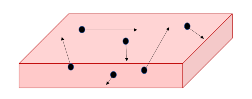
Since gravity is acting along the $z$ direction, we can use it as an analyzer since we can link the height obtained by an individual molecule to its kinetic energy, which then links to the initial speed. Since we won’t care, at this stage, about the horizontal components of each random motion, we’ll imagine that we’ve set them to zero and we’ll concentrate only on the vertical motion.
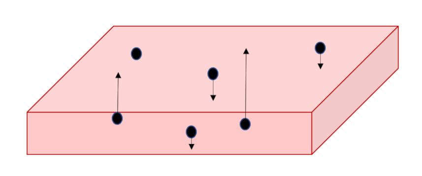
Since we seek the stationary distribution, we can further envision that there is a floor off of which the molecules can bounce keeping the supply of particles constant. These extracted particles will then separate into a thicker slab with the more energetic of them being able to obtain greater values in $z$ while the slower ones will remain at smaller heights; a vertical gradient in density will result solely due to differences in speed.
The next point in Boltzmann’s argument is point out that we know how to macroscopically describe such a density gradient in an isothermal atmosphere using fluid mechanics and thermodynamics. The first step is to start with the Euler equation (link) under the external influence of gravity
\[ \rho \frac{d}{dt} {\vec v} = \, – \nabla P + {\vec F}_g \; ,\]
where $\rho$ is the mass density. Specializing to stationary equilibrium in one dimension (called $z$, in keeping with the above argument):
\[ 0 = \, – \frac{d}{dz} P – \rho g \; . \]
The next step with a modification eliminating the mass density $\rho$ in favor of the number density $n$, to which it is proportional with the constant of proportionality being the molecular mass $m$: $\rho = m n$. The next step assumes the ideal gas law $P = n k_b T$ to eliminate the pressure giving
\[ \frac{dn}{n} = \, – \frac{m g}{k_B T} dz \; . \]
Since we’ve stipulated an isothermal profile (this assumption does not hold for the atmosphere as a whole it does for any local portion and that is all that is needed for Boltzmann’s argument to work), this differential equation readily solves to
\[ n(z) = n_0 \exp \left( – \frac{m g z}{k_B T} \right) \; , \]
where $n_0$ is some constant.
The next point in his argument is to relate the gravitational potential energy to molecules kinetic energy, thereby eliminating $z$. This is the point where the notion that the particles bounce vertical to different heights based on their initial velocities comes into play. This video by tec-science has a nice illustration of the physics. The final form for the number density as a function of $v_z$ is
\[ n(v_z) = n_0 \exp \left( – \frac{m v_z^2}{2 k_B T} \right) \; . \]
Demanding this function be normalized gives the distribution function
\[ f(v_z) = \sqrt{\frac{m}{2\pi k_B T}} \exp \left( – \frac{m v_z^2}{2 k_B T} \right) \; . \]
Boltzmann’s final point is that, although gravity was an essential part for getting started, now that it has been eliminated the form of $f(v_z)$ also applies to the $x$- and $y$-directions. The full three-dimensional form is
\[ f({\vec v}) = \left( \frac{m}{2\pi k_B T}\right) \exp \left( – \frac{m {\vec v}\cdot {\vec v}}{2 k_B T} \right) \; .\]
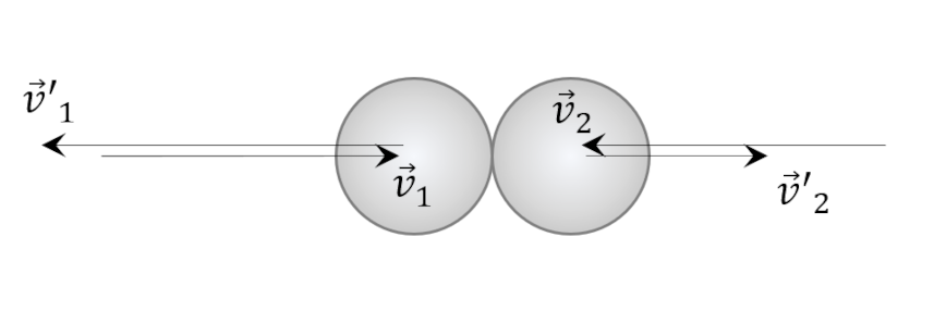
A different, physical approach is given by Carter in his Classical and Statistical Thermodynamics. To the usual kinetic theory assumptions, he adds the very plausible idea that in a dilute gas, only binary collisions are important. Similar to above, he limits the analysis to a single species of known mass $m$. The conservation of momentum requires
\[ {\vec v}_1 + {\vec v}_2 = {\vec v’}_1 + {\vec v’}_2 \; , \]
where ${\vec v}_1$ and ${\vec v}_2$ are the initial velocities of the two molecules and the primed versions are the final velocities.
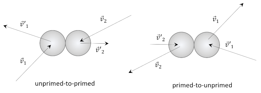
Carter points out that kinetic theory predicts that an inverse collision also has to be present taking ${\vec v’}_1$ and ${\vec v’}_2$ back to their unprimed versions in order to have equilibrium. He then assumes that $f({\vec v})$ is the distribution and that the number of collisions between molecules with velocity ${\vec v}_1$ and ${\vec v}_2$ is $\alpha f({\vec v}_1) f({\vec v}_2)$ for some constant $\alpha$. Likewise, the number of inverse collisions must be $\alpha’ f({\vec v’}_1) f({\vec v’}_2)$. As already remarked, in equilibrium
\[ \alpha f({\vec v}_1) f({\vec v}_2) = \alpha’ f({\vec v’}_1) f({\vec v’}_2) \; . \]
The final step involves recognizing that the two collisions, unprimed-to-primed and primed-to-unprimed, are equivalent in the center-of-mass frame (simply switch the arrow heads from in to out) so that $\alpha = \alpha’$.
Since the kinetic energy is conserved, the following constraint applies
\[ v_1^2 + v_2^2 = {v’}_1^2 + {v’}_2^2 \; .\]
After some reflection, one can see that the functional form
\[ f({\vec v}) = A \exp(-q {\vec v} \cdot {\vec v} ) \; \]
fits the bill. This is functionally the same distribution derived from the hydrostatic analysis above, although the values of $A$ and $q$ have not been determined yet. The form of $q$ follows from imposing a consistency constraint with the ideal gas law. Since the ideal gas law doesn’t involve directionality, we’ll find it convenient to construct a related distribution $f(v)$, which gives the fraction of the gas moving with speed $v$. This distribution is related to the velocity distribution by integrating over the angular degrees of freedom in spherical polar coordinates.
\[ f(v) = \int_0^{2 \pi} d\phi \int_{-1}^{1} d(cos(\theta)) v^2 dv A e^{-q {\vec v} \cdot {\vec v}} \\ = 4 \pi v^2 A e^{-q {\vec v} \cdot {\vec v}} \; . \]
Normalizing $f(v)$, over the range $[0,\infty)$, yields the relationship
\[1 = 4 \pi A \left( -\frac{d}{dq} \right) \frac{1}{2} \sqrt{ \frac{\pi}{q} } = A \left( \frac{\pi}{q} \right)^{3/2} \; .\]
Now we demand that the average of the kinetic energy $1/2 m v^2$
\[ \left< \frac{1}{2} m v^2 \right> = \int_0^{\infty} \frac{1}{2} m v^2 \times 4 \pi A v^2 e^{-q {\vec v} \cdot {\vec v}} \; . \]
be equal to $3/2 k_B T$, in keeping with the ideal gas law. Performing the appropriate integral yields
\[ \frac{3}{2} k_B T = \left( -\frac{d}{dq} \right) 2 \pi m A \left( \frac{\pi}{q} \right)^{3/2} = \frac{3 m}{4} A \frac{{\pi}^{3/2}}{q^{5/2}} \; , \]
or
\[ k_B T = \frac{m A}{2} \left( \frac{\pi}{q} \right)^{3/2} \frac{1}{q} \; . \]
Combining this relation with the normalization relation gives
\[ q = \frac{m}{2 k_B T} \; . \]
Another approach involves calculating the pressure and comparing against the ideal gas law also gives
\[ q = \frac{m}{2 k_B T} \; , \]
from which follows the same form as above. A nice derivation of this result comes from Heat and Thermodynamics by Anandamoy Manna.
This final form is
\[ f(v) = 4 \pi \left( \frac{m}{2 \pi k_B T} \right)^{3/2} v^2 \exp \left( – \frac{m v^2}{2 k_B T} \right) \; .\]
This is the famous Maxwell-Boltzmann distribution. In the next post, we’ll explore some of the consequences of this distribution.