
Kinetic Theory 3 – Exploring the Maxwell-Boltzmann Distribution
In this post, we explore some of the physical implications of the Maxwell-Boltzmann speed distribution
\[ f(v) = 4 \pi \left( \frac{m}{2 \pi k_B T} \right)^{3/2} v^2 \exp \left( – \frac{m v^2}{2 k_B T} \right) \; \]
derived in the previous post.
The first thing to note is that the decaying exponential favors lower speed (in the limit as $v \rightarrow \infty$, $f(v) = 0$) while the factor of $v^4$ favors higher ones ($f(v=0) = 0 $). As a result, we expect that there is a peak in the distribution somewhere between these two extremes. To verify this, we can plot $f(v)$ for the case where $m$ is the mass of a nitrogen gas molecule ($m_{N_2} \approx 28 Da$, where $1 Da \approx 1.66 \times 10^{-27} \, kg$) and the temperature is $300 K$, corresponding, roughly, to room temperature.
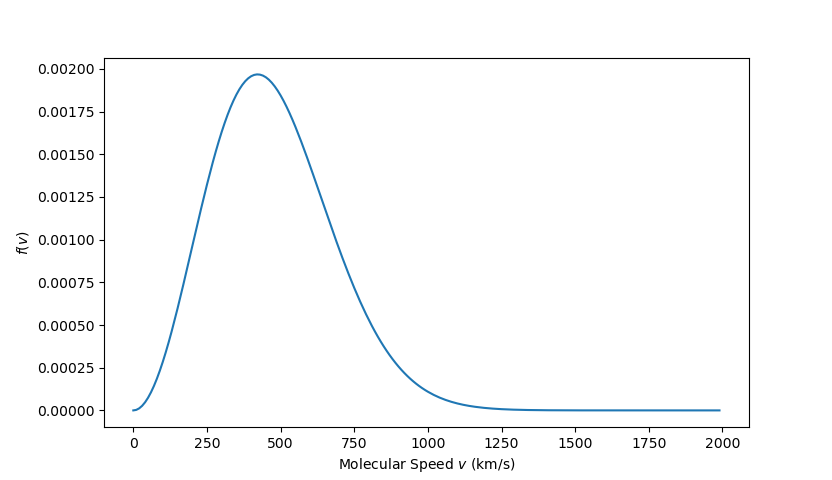
There is a distinct peak, which can be estimated by eye, at approximately $420 \, km/s$. This value is of the order-of-magnitude of the RMS speed given by
\[ v_{RMS} = \sqrt{ \frac{3 k_B T }{m_{N_2}}} = 510.77 \, km/s \; ,\]
but is substantially smaller by about $20 \, %$. The exact value at the peak, which corresponds to the most probable value, comes from finding the maximum of the distribution in the usual way. First we differentiate the distribution with respect to $v$ to get
\[ \frac{d f(v)}{d v} = 4 \pi \left( \frac{m}{2 \pi k_B T} \right)^{3/2} \left( 2 v – \frac{ m v^3}{k_B T} \right) \exp \left( – \frac{v^2}{2 k_B T} \right) \; . \]
Setting this expression to zero and solving for $v$ yields the most probable speed
\[ v_{mp} = \sqrt{\frac{2 k_B T}{m} } \; .\]
Plugging in the numerical values used above gives $v_{mp} = 417.04 \, km/s$, which is consistent with eyeball estimate of $420 \, km/s$.
The final speed of interest is the average speed defined by
\[ v_{ave} = \int_0^{\infty}\, dv \, v f(v) \; .\]
Ordinarily, the odd moment of any Gaussian-like distribution would be zero (e.g., the average of any component of the velocity would be zero – see last post) but since the speed is confined to the interval $[0,\infty)$, the integral yields a finite value. To get that moment, we start with
\[ J_1 = \int_0^{\infty} \, v e^{-qv^2} dv = \frac{1}{2} \int_0^{\infty} \, d(v^2) e^{-q v^2} \; .\]
Substituting $w = v^2$ yields a simple integral
\[ J_1 = \frac{1}{2} \int_0^{\infty} \, dw e^{-q w} = \frac{1}{2q} \; . \]
Higher order moments come by differentiation with
\[ J_3 = \int_0^{\infty} v^3 e^{-q v^2} dv = -\frac{d}{dq} \int_0^{\infty} v e^{-q v^2} = -\frac{d}{dq} \frac{1}{2q} = \frac{1}{2q^2} \; , \]
which, up to some constants, is the desired result.
Using this result, we arrive at the expression
\[ v_{ave} = 4 \pi \left(\frac{m}{2 \pi k_B T}\right)^{3/2} \frac{k_B T}{m} = \sqrt{ \frac{8 k_B T}{\pi m}} \; .\]
Plugging in the numerical values used above gives $v_{ave} = 470.58 \, km/s$, which falls between the most probable and the RMS speeds. We can annotate the graph with these three lines to draw out the distinctions
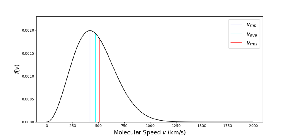
and we can note that the average speed is about $12.8 \, %$ higher than the most probable speed while the RMS speed is $22.5 \, %$ higher.
The final point to be explored is how the curve shifts as a function of temperature. Since all the speeds have the same functional form, differing only in the numerical coefficient, it is straightforward to see that each speed scales as $\sqrt{T}$. However, the overall shape of the curve can be a little surprising, which the following plot illustrates by looking at broad range of temperatures.
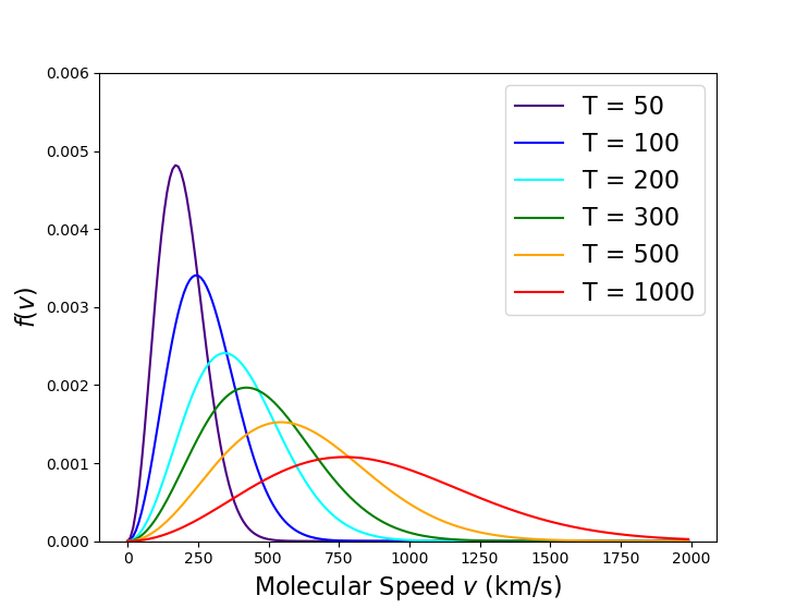
As the temperature increases, the distribution tends to being more symmetric by shifting right, effectively eating into the long tail.
Of course, the Maxwell-Boltzmann distribution is physically unrealizable as there is always a finite probability for having a speed equal or greater to the speed of light. But this is of little concern as very little of the distribution is found at these higher speeds. For example, the vast majority of the distribution is found below $2000 \, km/s$, which is $ < 0.01 c$, even at $T = 1000 K$.