
Kinetic Theory 4 – Mean Free Path
Having explored some of the numerical properties of the Maxwell-Boltzmann distribution and the various statistically significant speeds (RMS, most probable, mean), we now turn to the idea of the mean free path and the corresponding collisional frequency. Since the basic idea of kinetic theory is the mechanical interpretation of macroscopic thermodynamics it is natural to ask about what can be said statistically about the how far, on average constituent particles (e.g., gas molecules) travel before they collide with each other (mean free path) or how often they suffer a collision (collisional frequency).
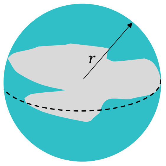
While the notion of the mean free path is simple enough, its computational form is difficult to come by. The reason for this is that it depends on one unknown parameter, the characteristic size of a particle. Typically, whether warranted or not, the particles are, for mathematical simplicity, assumed to be spherical and the so the characteristic size can be thought of as the radius of the bounding sphere into which the particle just fits.
The second complication is that the particles are all moving with various speeds distributed according to the Maxwell-Boltzmann distribution and it isn’t, a priori, obvious whether the mean free path depends on one of the statistically significant speeds or on the distribution as whole.
The content of this post follows, in certain areas, the discussions in Physics by Halliday and Resnick, Classical and Statistical Thermodynamics by Carter, and the Youtube video Mean Free Path by Steven Stuart for Physical Chemistry. All three agree that the first place to start is by focusing on one particle that is allowed to move within a frozen background of the rest.
Since each particle has a characteristic radius $r$ (and mass $m$), a collision will occur when any two particles are a distance $2r$ from each other.
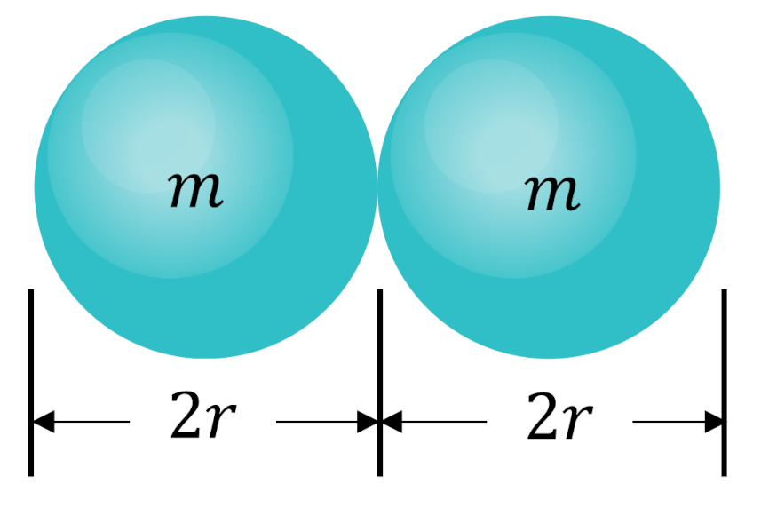
Mentally, we can then throw away the bounding sphere around each of the frozen particle, replace the bounding sphere around the mobile particle with one twice as large, and then ask how many particle centers are contained in the cylindrical volume swept out as the mobile particle moves.
The cross-sectional area of this cylinder is $A = \pi (2r)^2$. If the mobile particle moves a distance $\lambda$, then the volume is
\[ Vol = \lambda A = \lambda \pi 4 r^2 \; . \]
The average number of frozen particle centers that fall within this volume, $N_c$, depends on the number density as
\[ N_c = Vol \cdot n = \lambda \pi 4 r^2 n \; .\]
By definition, the mean free path is the distance, on average, a particle moves before suffering its first collision. Setting $N_c = 1$ then gives the first estimate as
\[ \lambda = \frac{1}{4 \pi r^2 n} = \frac{1}{\pi d^2 n} \; , \]
(where $d = 2r$) which is the result that all three references agree on.
This result can only be justified under the original assumption of one mobile particle moving in a fixed background of all the others being anchored in place. So, while the above result is dimensionally correct (i.e., the dependence on $(d^2 n)^{-1}$) the prefactor might be different.
To get a sense of how this prefactor might differ, Halliday and Resnick actually argue for the above result differently. They assign the mobile particle a speed $v$ and argue that the length it travels in elapsed time $t$ is $vt$. The total number of collisions is again $\pi d^2 n v t$ and the ratio of these two expressions gives the mean free path
\[ \lambda = \frac{v t}{\pi d^2 n v t} \; . \]
Of course, with the assumption of a single mobile particle, the speeds in the numerator and denominator are identical and can be cancelled out giving the expression derived earlier. But once we free the previously anchored-in-place particles to move, one must distinguish between the speed in the numerator, which is the “average” speed with respect to the lab (i.e., with respect to the walls of the enclosure) while the speed in the denominator is the speed of the particle we are focusing on relative to the others. The mean free path now can be written as
\[ \lambda = \frac{v_{avg}}{\pi d^2 n v_{rel}} \; . \]
This argument is a bit subtle and it’s open to interpretation, at this point, which of the statistically significant speeds corresponds to $v_{avg}$ and it is for this reason that not every text agrees on exactly how to determine the ratio of $v_{avg}/v_{rel}$.
At this point, it is worth reminding ourselves that all the statistically significant speeds, $v_{ss}$, take the form of
\[ v_{ss} = N \sqrt{\frac{k_B T}{m}} \; , \]
where $N = \sqrt{2}$ for most probable, $N = \sqrt{8/\pi}$ for mean, and $N = \sqrt{3}$ for RMS. (It seems the best mnemonic is that $N^2$ is 2, 2.5, and 3, since $8/\pi$ is approximately 2.5 with only a 1.9
Thus, we can eliminate a common factor of $\sqrt{k_B T}{m}$ from the numerator and denominator to arrive at
\[ \lambda = \frac{1}{(N_{rel}/N_{avg}) \pi d^2 n} \; .\]
While he doesn’t reduce to the analysis as has been done here, Stuart points out that the resulting expression for the mean free path should have some traces of the speed lingering around when everyone is moving. He gives two examples in which all the particles have the same speed. He argues if all the particles are moving coherently in the same direction, then the relative velocity is zero and there will be no collisions. Alternatively, if one of them is moving oppositely to the others, the number of collisions for this one particle must be double what was predicted by the naïve result. This is the same argument given in Halliday and Resnick. Stuart then goes on to derive the correction as follows.
First look at the relative velocity between particles A and B such that
\[ {\vec v}_{rel} = {\vec v}_A – {\vec v}_B \; .\]
Squaring both sides and averaging over all pairs of particle A and B gives
\[ \langle v_{rel}^2 \rangle = \langle v_{A}^2 \rangle + \langle v_{B}^2 \rangle – 2 \langle {\vec v}_A \cdot {\vec v}_B \rangle \; .\]
Since we envision a large number of particles, the last term averages to zero and we are left with
\[ \langle v_{rel}^2 \rangle = 2 \langle v^2 \rangle \; \]
or
\[ v_{rel,RMS} = \sqrt{2} v_{RMS} \; .\]
With this result, $N_{rel}/N_{avg} = v_{rel,RMS}/v_{RMS} = \sqrt{2}$ and the expression for the mean free path is
\[ \lambda = \frac{1}{\sqrt{2} \pi d^2 n } \; .\]
Interestingly, this is not the expression derived by Carter. In Sec. 11.7, he states
Frankly, it isn’t quite clear what he means, and the best interpretation seems to be that the relative speed is $\sqrt{2}$ larger than the mean speed (the extra factor most likely due to considerations similar to the above) the while the average speed is identified with the most probable speed (an assumption further supported by his use of the most probable speed in calculating the collision frequency). With these assumptions the ratio
\[ \frac{v_{avg}}{v_{rel}} = \frac{\sqrt{2 k_B T/m}}{\sqrt{2}\sqrt{8/\pi k_B T/m}} = \frac{1}{\sqrt{8/\pi}} \; .\]
In the end, this minor distinction ($\sqrt{2}$ vs. $\sqrt{2.5}$) doesn’t matter (beyond clarity and pedagogy) since the there is no way to know, with certainty, what the particle diameter $d$ actually is and these formulae are usually used to infer $d$ by measuring $\lambda$.
Next column will look at some characteristic values and the corresponding question of the collision frequency, where, again, we’ll have to wrestle a bit with which of the statistically significant speeds to use.