
Hard Sphere Gas – Part 2: Simulation
Last month’s blog presented the theory of a motion of a hard sphere gas confined to a box with the following three physical effects being modeled: 1) free propagation between collisions, 2) elastic collisions with the walls of the box, and 3) elastic collisions with each other. In this month’s post, a python simulation uses these results to model the approach to thermalization and the Maxwell Boltzmann speed distribution are discussed and the results are presented.
As state last month, the resulting simulation is heavily influenced by the HardSphereGas-VPython simulation by Bruce Sherwood over at Glowscript.org, although certain tweaks and corrections have been made and the code is entirely a new rewrite. The image below is taken from one moment in his simulation:
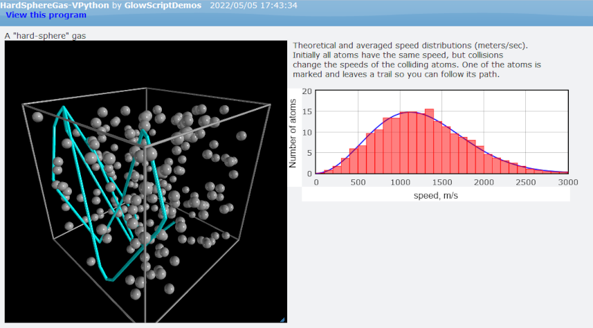
Following Sherwood, each hard sphere in the gas is initialized to have the same kinetic energy based on the temperature being modeled using the standard kinetic theory result
\[ v = \sqrt{ \frac{3 k_b T}{m} } \; . \]
However, their positions components are randomly assigned to be uniformly distributed within the confining box of side length $L = 1 m$. The directions are also randomly assigned by drawing values for the polar and azimuthal angles describing each sphere’s unit vector from uniformly over the intervals $[0,\pi]$ and $[0,2\pi)$, respectively.
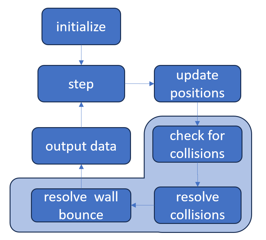
Once initialized, the simulation turns to evolving the gas step-by-step as time elapses. Although this evolution is an instance of Newton’s laws, the position and velocity updates do not need to be solved-for simultaneously as is the case for more complicated dynamics. The time step simulation consists of four parts: 1) incrementing of time, 2) updating of positions, 3) updating of velocities, and 4) outputting of data at each time step for subsequent analysis. Only step 3) is particularly involved. It consists of three sub-steps: 3a) check for any collisions that have occurred due to the position update, 3b) a resolution of the collisions between the hard spheres using the center-of-momentum formulae develop in the previous post, and 3c) the resolution of any collisions with the walls using the reflection formula also developed last month.
The method for implementing step 3) involves first scanning the new positions resulting from step 2) to look for any overlaps defined by the condition $ |{\vec r} | < 2 R$, where $|{\vec r}|$ is the relative distance between each distinct pairs of particles. The indices of two particles for which this condition is true are appended to a hitlist for subsequent resolution.
Once the hitlist is completely populated, collisions are resolved pairwise by:
- first determining what negative time step, $\delta t$, to apply to bring the particles to an earlier time when they would have just touched
- stepping backwards to that time using same formula for updating positions
- adjusting the momenta/velocities of the particles to simulate the hard sphere bounce
- moving the particles forward in time by the same $\delta t$ amount
The following animation shows one such encounter.
Since, while rare, there is no way to preclude an overlap of three of more hard spheres, the condition that $|{\vec r}| < 2 R$ must be subsequently checked again for each pair as the resolution of an earlier collision may have also resolved the other overlaps. This approach for resolving ternary or higher collisions is entirely unphysical but only modestly unsatisfactory because it is so rare (34 cases out of 10,000 in one simulation) that its influence on the physics is small. That said, it drives home that one area where our current understanding of physics is lacking is in a general understanding of complicated multibody situations where ternary or more complicated interactions are common.
Finally, the particles are checked for exceedances beyond the confines of the box and, when found to have happened along one of the Cartesian axes, the normal component of the corresponding velocity is negated and the particles component is adjusted as explained in last month’s post. Of course, this position adjustment could also create new overlaps but these are also rare and so are not checked for.
In the last step, the speeds of the particles are put into a row of a numpy array which is outputted for subsequent analysis.
I mostly used the same simulation parameters as Sherwood, modeling the particles as ‘fat’ helium atoms with a molar mass of 4 grams and a radius of 30 millimeters (very fat) at a temperature of 300 K. Once initialized, the simulation was run for 2000 time steps.
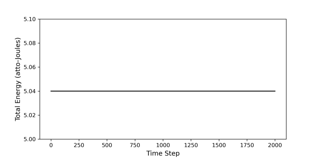
The first check on the goodness of the simulation was to plot the time history of the total energy of the particles $E = \sum_i 1/2 m_{He} {v_i}^2$. Since the collisions between the hard spheres and the walls and with each other are elastic, the energy should be conserved as it clearly was as seen in the following plot.
The next measure was to look at the time evolution of the speed statistics for the average, the maximum, and the minimum over the 400 particles. The following plot shows their respective values showed no secular trends but did shows fluctuations from time step to time step, with the most pronounced being in maximum and the least in the average.
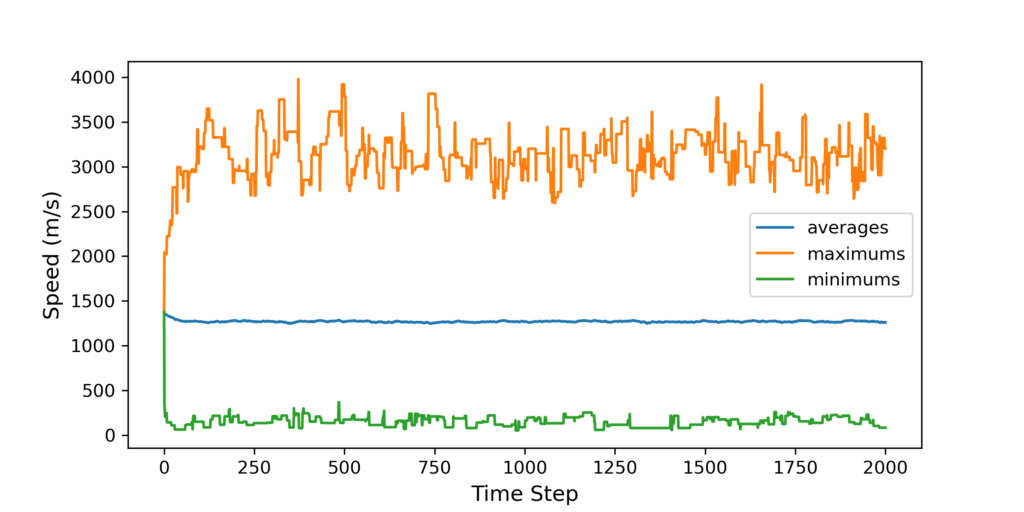
These results are consistent with our expectations since the maximum speed is virtually limitless while values around the average will be populated with a large number of particles tending to smooth out variations.
Far more informative are animations of the time history of the instantaneous and time averages distribution of the speeds of relative to the theoretical Maxwell Boltzmann distribution (red curve).
In both cases, the initial distribution shows a single, populated bin due to all particles being initialized with the same speed. For the instantaneous distributions, the memory of this is quickly lost with most subsequent distributions fluctuating raggedly about the theoretical distribution.
These results closely match results on YouTube in the videos Simulation of an Ideal Gas to Verify Maxwell-Boltzmann distribution in Python with Source Code by Simulating Physics and Maxwell-Boltzmann distribution simulation by Derek Harrison.
For the evolution of the time average distribution, the memory of the initial, coherent distribution lingers but the fluctuations from time step to time step are smoothed.
It is here that we most clearly see the approach of the system to the Maxwell Boltzmann distribution. Of course, we expect that as the number of particles increases the qualitative differences between the instantaneous and time average animations to disappear. When this occurs the system is said to have reached the thermodynamic limit.