
Boltzmann Equation – Part 1: Basic Theory
This month’s post begins the study of phase space density $f$ and Boltzmann’s and related equations that govern its evolution. The arrangement and approach closely follows the heuristic derivation in the Eulerian picture by Prof. Jeffrey Freidberg in Lecture 1 of his MIT OpenCourseWare class on magnetohydrodynamics. Next month’s blog augments this analysis with my own clarifications based in the Lagrangian picture and Liouville’s theorem.
The main actor in our drama is the phase space density, $f({\vec r},{\vec v},t)$, which tells us what fraction of the total number of particles $N$ that we have in our system can be found localized to a small volume $\Gamma$ centered on position ${\vec r}$ and velocity ${\vec v}$:
\[ N_{\Gamma} = f({\vec r},{\vec v},t) \, \Gamma = f({\vec r},{\vec v},t) \, d^3r \, d^3v \; . \]
We assume that $f$ depends not only where one is at in phase space but also that it may, and generally does, vary in time. Since $f$ represents a fractional quantity many people interpret $f$ as a probability density function but I find it much more convenient to simply think of it as a type of continuum approximation (i.e., fluid) of the underlying collection of discrete, delta-function like, compactly supported kernels corresponding to the individual particles making up the gases, liquids, and plasmas to which this formalism is typically applied. The distinction is negligible for liquids but becomes increasingly importantly for rarefied gases and plasmas, particularly in space physics where the particle density $n({\vec r})$ (as we’ve used in past posts on kinetic theory) becomes very low (typically $< 1/cm^3$).
Freidberg starts the derivation of the Boltzmann equation for phase space density as one does the continuity equation of ordinary number density in fluid mechanics by equating the temporal change in the number of particles $dN_{\Gamma}$ in an elementary, fixed phase space volume (thus the Eulerian picture) to the flux of particles flowing into and out of that small volume in some unit time plus the rate at which particles are created or destroyed within the volume $S$. Note that here we are assuming that particle number need not be explicitly conserved to account for effects like when a single particle, like an atom, is suddenly ionized into two pieces, producing an ion and an electron.
The hardest part of Freidberg’s derivation is to recognize how to generalize the ordinary flux of fluid mechanics to the proper form of the flux ${\vec \phi}_{\Gamma}$ in phase space. In ordinary fluid mechanics, particles can flow into or out of a physical volume carried by the velocity. In phase space, particles can flow into and out of the velocity volume carried by the acceleration. We’ll examine this process explicitly in a phase space of 2 dimensions $\Gamma = dx dv_x$ centered at a point $(x,v_x)$.
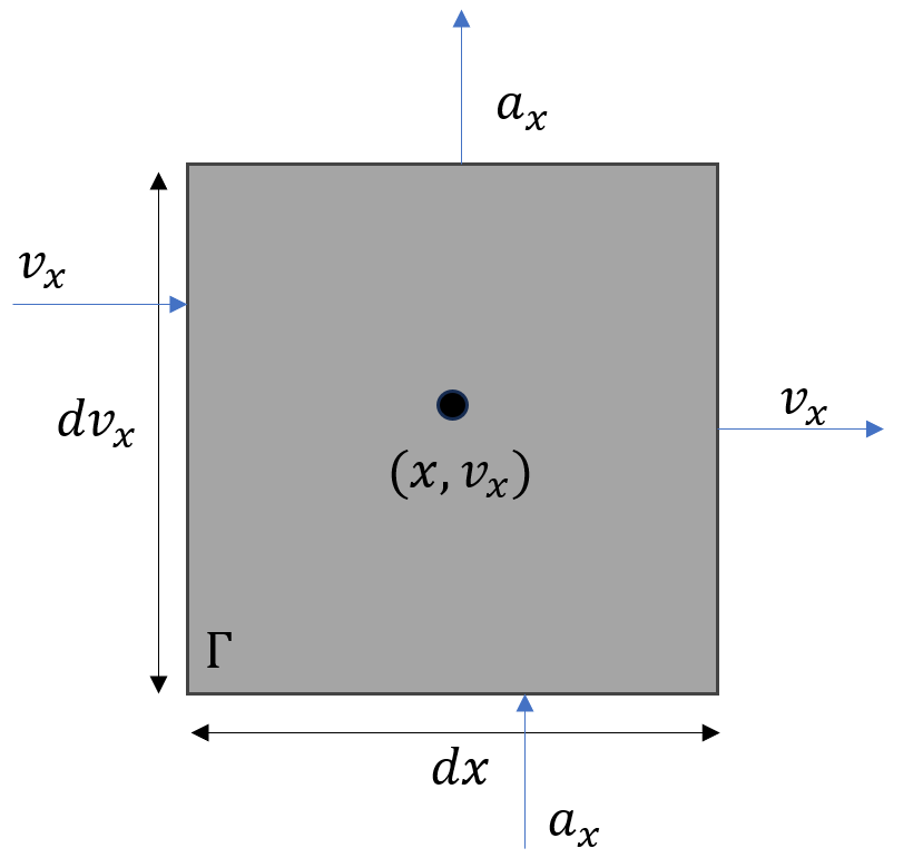
The number of particles that flow out of $\Gamma$ on the four sides in the interval of time $dt$ is given by
\[ dN_{\partial \Gamma} = \sum_{i = 1}^4 {\vec \phi}_{\Gamma}(side_i) \cdot {\hat n}_i \, dA_i \, dt \; , \]
where ${\hat n}_i$ and $dA_i$ are the outward normal and the area of the ith side and the notation $\partial \Gamma$ reminds us that the change is particle number is due to the flow across the boundary of $\Gamma$. Since the flux is given by particles that are carried by the velocity $v_x$ into or out of the spatial faces of the volume or are carried by the acceleration $a_x$ into or out of the ‘velocital’ faces of the volume (to coin a phrase) the mathematical form of the flux is
\[ {\vec \phi}_{\Gamma} = f(x,v_x,t) \left[ v_x(t) {\hat x} + a_x(x,v_x,t) {\hat v}_x \right] \; .\]
Since we are working in a Eulerian picture in a phase space, the velocity flow piece of the flux does not have any spatial dependence. Freidberg notes this point in passing when he says at the bottom of page 3
Note that $\partial v_x/\partial x = 0$ (independent coordinates)
This is in marked contrast to the usual equations of fluid mechanics where the velocity has a spatial dependence that ultimately explains the $\partial (\rho v_x)/\partial x$ term in the usual continuity equation.
Substituting this expression into the one above and taking care to use the outward normal on the four faces we get our total flow of particles into and out of $\Gamma$. However, the expression is a bit unwieldy and it is cleaner to examine the spatial contribution, $dN_{\partial\Gamma;x}$, separately from the ‘velocital’ one, $dN_{\partial\Gamma;v_x}$.
The spatial portion is
\[ dN_{\partial \Gamma;x} = \left[ f(x+\frac{dx}{2},v_x,t) – f(x-\frac{dx}{2},v_x,t) \right] v_x(t) \, dv_x \, dt \; . \]
Expanding and keeping terms (with the functional dependence suppressed) only to first order gives
\[ dN_{\partial \Gamma;x} = \frac{\partial f}{\partial x} v_x \, dx \, dv_x \, dt \; . \]
The ‘velocital’ portion is
\[ dN_{\partial \Gamma;v_x} = \left[ f(x,v_x + \frac{dv_x}{2},t) a_x(x,v_x + \frac{dv_x}{2},t) \\ – f(x,v_x – \frac{dv_x}{2}) a_x(x,v_x – \frac{dv_x}{2},t) \right] dx \, dt \]
Again, expanding and keeping terms (again with the functional dependence suppressed) only to first order gives
\[ dN_{\partial \Gamma;v_x} = \frac{\partial (f a_x)}{\partial v_x} dx \, dv_x \, dt \; . \]
Adding these pieces together gives
\[ dN_{\partial \Gamma} = \frac{\partial f}{\partial x} v_x dx dv_x + \frac{\partial (f a_x)}{\partial v_x} dt \, dx \, dv_x \; . \]
The total change in the number of particles within the volume due sinks and sources is
\[ dN_{S} = S dt \, dx \, dv_x \; \]
where $S$ is the rate at which particles are created or destroyed.
The contributions from these two terms has to equate with the change of the number of particles within the volume; that is to say
\[ dN_{\Gamma} + dN_{\partial \Gamma} = dN_{S} \; . \]
But the definition of $f$ allows the left-hand side to be expressed in terms of the time rate of change of the phase space density over a time interval $dt$ as:
\[ dN_{\Gamma} = \frac{\partial f}{\partial t} dt \, dx \, dv_x \; . \]
Substituting all of these pieces in yields
\[ \frac{\partial f}{\partial t} + \frac{\partial f}{\partial x} v_x + \frac{\partial (f a_x)}{\partial v_x} – S = 0 \; . \]
This equation has the immediate generalization to
\[ \frac{\partial f}{\partial t} + \nabla f \cdot {\vec v} + \nabla_v \cdot (f {\vec a}) – S = 0 \; . \]
It is traditional to expand the acceleration term as
\[\nabla_v (f {\vec a}) = (\nabla_v f) \cdot {\vec a} + f \, (\nabla_v \cdot {\vec a}) \; \]
and then to take the velocity gradient of the acceleration and source-sink term $S$ to the other side to arrive at
\[ \frac{\partial f}{\partial t} + \nabla f \cdot {\vec v} + (\nabla_v f) \cdot {\vec a} = – f \, (\nabla_v \cdot {\vec a} ) + S \; . \]
Collectively, the terms on the left-hand side represent the material derivative of $f$ along a particular trajectory in phase space while the right-hand side can be thought of as collisions (i.e. momentum transfer). Much of modern kinetic theory is devoted to understanding, interpreting, and explicitly expressing these terms.
As an example of how this analysis is done, Freidberg states that for a plasma “[i]n most cases of interest ${\vec a}$ can be divided into two parts”, which he denotes as ${\vec a} = {\vec a}_s + {\vec a}_l$ with the first term being due to short-range forces and the second being due to long-range ones. Arguing that Debye screening eliminates ${\vec a}_s$ and that the form of the long-range acceleration is the Lorentz force-per-mass due to the average or mean electric and magnetic fields, Frediberg arrives at
\[ {\vec a}_l = \frac{q}{m} \left( {\vec E} + {\vec v} \times {\vec B} \right) \; . \]
The interesting consequence of this assumption is that, despite the presence of an explicit factor of the particle velocity within the expression, $\nabla_v \cdot {\vec a}_l = 0$. This can be seen as follows:
\[ \nabla_v \cdot {\vec a}_l = \frac{q}{m} \nabla_v \cdot \left( {\vec E} + {\vec v } \times {\vec B} \right) = \frac{q}{m} \nabla_v \cdot \left( {\vec v} \times {\vec B} \right) = \frac{q}{m} {\vec B} \cdot (\nabla_v \times {\vec v}) = 0 \; . \]
The consequence of these assumptions (and an additional assumption he does not explicitly state that $S=0$) is that the right-hand side of the Boltzmann equation is identically zero and we are left with the Vlasov equation for a collisionless plasma
\[ \frac{\partial f}{\partial t} + \nabla f \cdot {\vec v} + \frac{q}{m} \left({\vec E} + {\vec v} \times {\vec B} \right) \cdot (\nabla_v f) = 0 \; . \]