
Circular Restricted Three Body Problem – Part 3: Initial Exploration of the Pseudo-potential
Last month we derived Jacobi’s pseudopotential $U$ for the circular restricted three body problem. In the co-rotating frame, the pseudopotential takes the form:
\[ U = \frac{1}{2} \left( x^2 + y^2 \right) – \frac{1-\mu}{d_1} – \frac{\mu}{d_2} \; , \]
where $d_1$ and $d_2$ are the distances between the restricted body and the location of the primary and secondary bodies, respectively, which are given by
\[ d_1 = \sqrt{ (x+\mu)^2 + y^2 + z^2 } \; \]
and
\[ d_2 = \sqrt{ (x-1+\mu)^2 + y^2 + z^2 } \; . \]
Despite the fact that the underlying equations of motion are non-autonomous, there is a conserved quantity, called the Jacobi constant $C_J$, that exists in the co-rotating frame such that
\[v^2 = 2U – C_J\; .\]
This very innocent looking expression holds a number of important results if we know how to mine it.
We’ll start our interrogation with a visual inspection of the magnitude of $U(x,y,0)$, which corresponds to the value of the potential in the orbital plane of the massives. We will also set the mass fraction $\mu=0.5$ meaning that the primary and secondary are of equal mass and that the barycenter or center-of-mass around which they orbit is halfway along on the line joining them from either one.
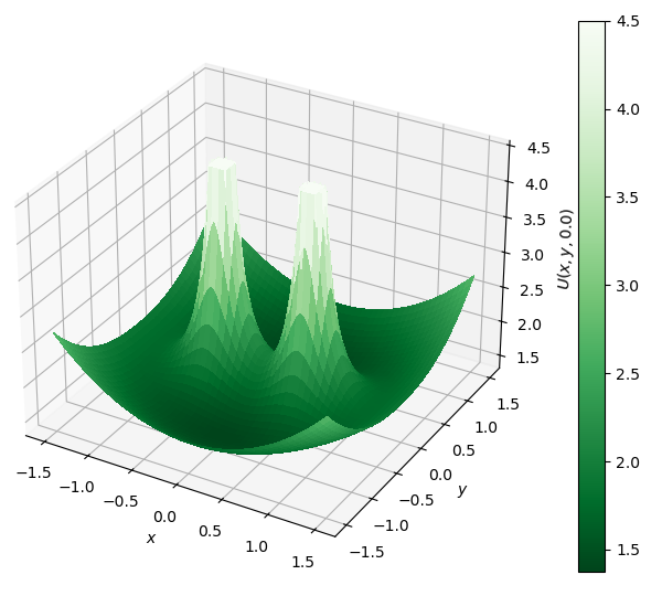
There are a number of things to note about this surface plot. Where the distance from the origin is large the edges of the plot are curling upwards. This is because at large values of $x$ or $y$ the quadratic term in the pseudopotential dominates and far from the origin, the surface will look, if one doesn’t squint too hard, like a paraboloid of revolution. The behavior is a manifestation of centrifugal force which arises in the rotating frame. Near each of the massives, the pseudopotential spikes sharply. For the purposes of the plot, the maximum value has been capped at a value of 4.5 but the function itself is unbounded the closer the restricted particle gets to the center of the either massive.
Due to the definition of the Jacobi constant $C_J = 2U – v^2$, and somewhat contrary to a conventional surface in the presence of uniform gravity, upward curvature in the surface plot of $U$ represents an instability. This observation is particularly relevant along the line joining the massives. Careful inspection will show that point half-way between them is a saddle point with upward curvature along the $x$-direction and downward curvature along $y$. After placing the restricted particle at the origin, we can ask what will happen if that particle is displaced a bit in one direction or the other. Displacement by a small amount in $x$ causes the restricted particle to fall towards whichever of the two massives is closer. Displacement by a small amount in $y$ causes the restricted particle to oscillate back and forth through the origin.
A better understanding of this dynamic behavior comes from first stepping back to a much simpler problem. Imagine that we start with two equal masses that are fixed in space rather than being free to co-orbit their center-of-mass. Next, let’s place our restricted body into this scenario in the region between the two bodies and examine the forces, ${\vec F}_1$ and ${\vec F}_2$.
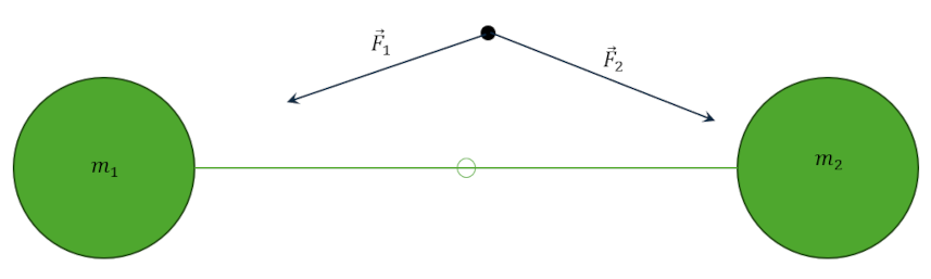
When the restricted body reaches the origin, which is the only point of symmetry in this problem, the forces exerted by each of the massives are equal and opposite. If we place the restricted body there at rest it will stay there at rest (i.e., in equilibrium) since no net force exists to move it anywhere else. Should we displace the restricted body in a plane perpendicular to the line joining the massives (which we will call hereafter the center line) the component of the forces along the center line will cancel but the perpendicular components will add. The action of the net force is to produce a restoring force back to the origin. A particle so displaced will oscillate in that plane, starting from rest at the furthest distance from the origin it can reach (i.e., the turning points) and accelerating to the origin. It’s kinetic energy will cause it to shoot past the origin and reach a turning point exactly the same distance but oppositely directed across the center line. So far so good. It is only when the particle is displaced along the center line that we see trouble in paradise. In this scenario, the closer of the two massives now exerts a force with a component along the center line that is larger than the other. The net force continues to accelerate the particle away from the origin and towards the closer of the two massives. In this way, we can come to understand that the origin, which is the point halfway between the two massives (remember $\mu=0.5$ in this case) is an unstable equilibrium point and that the plane perpendicular to the center line and which contains the origin is a stable subspace in which the particle can oscillate in bounded motion. But, as soon as the particle is displaced even minutely from this plane it will rush towards the closest of the two massives.
To transition from this idealized fixed mass scenario to the true circular restricted three body problem comes by regarding the frame as the rotating frame and taking into account the centrifugal force. Since that force is always directed radially outward from the origin, 4 new equilibrium points arise as places where the inward pull of gravity due to both bodies balance the outward pointing centrifugal force. Note that at the origin the centrifugal force is zero so the above argument is unaffected. The following contour plot shows the shape of different values of $U(x,y,0)$ and the yellow dots denote schematically the location of the 5 equilibria.
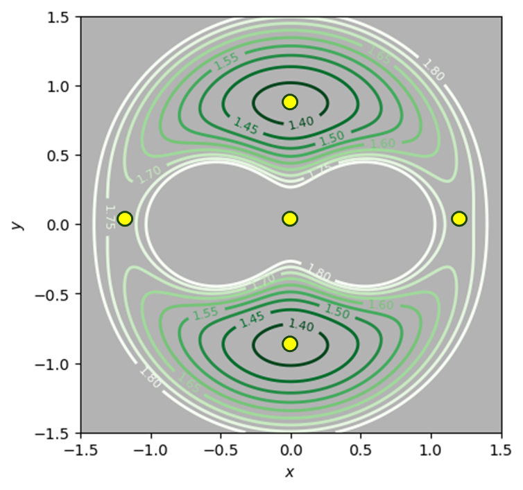
As an example, the equilibrium point on the right that falls on the center line exists because both massives are tugging the particle to the left while the centrifugal force pulls it to the right. The same hold true for the other equilibria with the obvious changes for direction. The saddle curvature of $U(x,y,0)$ at the origin and the open ‘figure eight’ shape of the contour line surrounding the massives reflect the mixed equilibrium at the origin. The contour plot indicates that the other two equilibrium points on the center are also mixed (also called unstable) equilibria. The interpretation for the two points is not as obvious and we will deal with them (and the colinear points as the other three are called) in later posts.
For now, we have a heuristic understanding of how equilibria arise at special locations in space based on the geometry of the pseudopotential. Next month, we will quantitatively explore the interaction between the $U$ and the velocity of the particle in the rotating frame as governed by $2U = C_J + v^2$ where we will see how the geometry of $U$ and the value of Jacobi’s constant allows us to make global predictions as to the allowed regions in which the restricted particle can move.