Uncategorized

A New Direction on Vectors

This post grew out of a discussion I had with my son who is now learning physics at the high school level.  He was reading his text book with the old, time-honored discussion of vectors being things with directions and magnitudes.  This is certainly true for physical vectors that describe things like displacement, velocity, force, torque, and electric and magnetic fields – all the typical menagerie that introductory physics students encounter.

But I couldn’t resist talking to him about vector spaces in general.  It has long baffled me why we teach kids from the beginning the dumbed-down version of things then make them unlearn it later on.  From what I can tell, the really creative thinkers of history were ones who didn’t succumb to this mind-numbing nonsense.  They were people who didn’t let the accepted way of doing things constrain them.  If they had, we would never have heard of them.

Thus I resolved to talk to him about vectors in general.  I introduced him to the rules for defining a vector space.  A short aside is warranted on this point.  Depending on which textbook you read, there are subtle differences in what is presented.  Some books enumerate only eight properties, some only seven, and the ones that do it best list 10.  All of them functionally amount to the same thing but standardization seems to elude the community at large, much to the confusion of students.

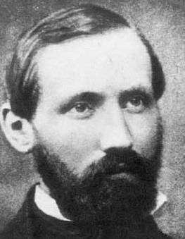
I touched on all the abstract definitions and properties just to show that there was a firm structure we could build on, but I emphasized that the prototype example of a vector that one could almost always use and never be led astray was a list.  I emphasized that what made the list useful was that it was a vector space in its own right and that almost all other vector spaces could be put into correspondence with a list.  I also emphasized that, while the list was helpful, it is often only a representation of the vector in question, and that we shouldn’t be seduced into thinking it was the vector itself.  A velocity vector is no more a list of numbers than Bernard Riemann is the list of pixels in the 2-array of light and shadow below.
Bernard_Riemann

We finished our discussion by touching on infinite-dimensional vector spaces, and I could see that what I really needed was a concrete example that he could play with.  After about an hour of back-and-forth I finally came up with something that he seemed to grasp.  I offer it here in the hopes that others will be able to use it as well.

What I wanted to create was a model where four properties were met:

  • The basic units are lists
  • These lists can be added component-wise
  • The lists can be infinite
  • The lists can be directly translated into a picture that visualizes magnitude and direction

A note is needed on the point that the lists can be infinite.  By this I mean that the length of the list was limited only by our patience and aesthetics or by the physical memory of the machine.  Much in the usual idea of infinity, I wanted a system where the student could always reach into the bag and pull out another dimension (being assured that the student would tire before the computer would).

The model that I created is expressed in the computer algebra system wxMaxima 11.08.0 running Maxima version 5.25.0. I like Maxima for several reasons, chief amongst them being that it is very capable and it is free.

Being based on LISP, Maxima is quite comfortable handling the first property.  For the second and third properties, I wanted a way to add lists of different lengths, so that the student would never encounter a limitation saying that one list was as long as another.  A different way of expressing that is to say that if there are two lists
\[ M = \left[ m_1, m_2, m_3 \right]\]
\[ N = \left[ n_1, n_2, n_3, n_4, n_5 \right]\]
they are not actually different in length since we can always imagine that they list only the portions of themselves beyond which there are only zeros (i.e. $$m_3$$ and $$n_5$$  are the last non-zero entries in their respective lists) so that they actually look like
\[ M = \left[ m_1, m_2, m_3, 0, 0, 0,…,0,… \right]\]
\[ N = \left[ n_1, n_2, n_3, n_4, n_5,0,…,0,… \right]\]
To do this I wrote a small Maxima function called add_lists that pads the smallest of the two lists with zeros and then returns the sum.  The code for it is

add_lists(a, b)  := block([ret_lst],
                      Na    : length(a),
                      Nb    : length(b),
                      delta : abs(Na-Nb),
                      pad   : makelist(0,i,1,delta),
                      if Na > Nb 
                         then ret_lst : a + append(b,pad) 
                         else ret_lst : append(a,pad) + b);

For the final property, I decided that a plot of a Fourier series in the interval $$[0,L]$$ would correspond to the visual addition of the vectors.

The particular choice of Fourier series is the cosine series given by
\[ f(x;L) = \sum_{n=1}^{\infty} a_n \cos \left( \frac{ 2 \pi n x}{L} \right) \; , \]
where the constant offset term given by $$a_0$$ has been set equal to zero and the presence of the term L there to remind us of the interval over which the function is defined.   Traditional treatments in advanced mathematics and quantum texts, drive the point that the sine and cosine function are orthogonal polynomials
\[ \int_0^{2 L} dx \cos \left( \frac{ 2 \pi n x}{L} \right) \cos \left( \frac{ 2 \pi p x}{L} \right) = \delta_{np} L \]
\[ \int_0^{2 L} dx \sin \left( \frac{ 2 \pi n x}{L} \right) \sin \left( \frac{ 2 \pi p x}{L} \right) = \delta_{np} L \; \; (n \neq 0)\]
\[ \int_0^{2 L} dx \cos \left( \frac{ 2 \pi n x}{L} \right) \sin \left( \frac{ 2 \pi p x}{L} \right) = 0 \]
in a Sturm-Liouville sense and thus are basis vectors in some abstract space.  The coefficients $$a_n$$ are then the components of the general vector (function)  in this space.  While important to the theoretical underpinnings, these relationships obscure what is really a rather simple concept that two sets of constants can be added together as a short hand for adding the two trigonometric series together and thus lists of these constants form a vector space in their own right.

Thus the list $$A = \left[a_1, a_2, …\right]$$ is the representation of the vector (in component or list form) and the function fourier_series given by

fourier_series( lst, L ) := block([expr],
                                  expr : 0,
                                  for i : 1 step 1 thru length(lst) do 
                                   ( temp_expr : lst[i]*cos(2*
                                     expr : expr + temp_expr ),
                                  expr);

is what delivers the corresponding expression that is plotted.

The final step is to take two lists, plot them separately to give the ‘direction and magnitude’ of each, and then to add them together plot-wise (that is to say plot the sum of the expressions) and show that the resulting vector is the same that is obtained if the two lists of coefficients are add together first and then plotted.

For a concrete example take the lists
\[A = \left[-1,\frac{1}{2},-\frac{1}{3},\frac{1}{4},-\frac{1}{5},\frac{1}{6},-\frac{1}{7}\right] \]
and
\[B = \left[1,\frac{4}{5},\frac{3}{5},\frac{2}{5},\frac{1}{5}\right] \; .\]

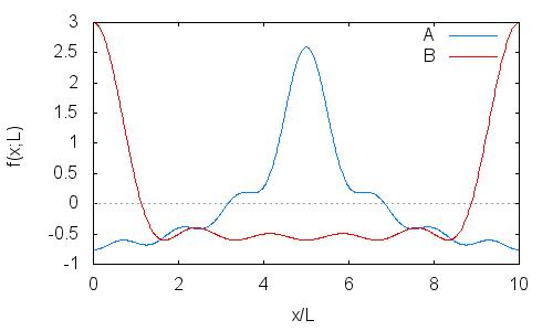
Lists $$A$$ and $$B$$ produce a plot of $$f_A(x;L)$$ and $$f_B(x;L)$$ over the interval $$x \in \left[0,L\right]$$
fourier_vector_plot_A_and_B
With corresponding expansions of fourier_series(A,L)
$$f_A(x;L) = -{{\cos \left({{7\,\pi\,x}\over{5}}\right)}\over{7}}+{{\cos \left({{6\,\pi\,x}\over{5}}\right)}\over{6}}-{{\cos \left(\pi\,x\right)}\over{5}}+{{\cos\left({{4\,\pi\,x}\over{5}}\right)}\over{4}}-{{\cos \left({{3\,\pi\,x}\over{5}}\right)}\over{3}}+{{\cos \left({{2\,\pi\,x}\over{5}}\right)}\over{2}}-\cos \left({{\pi\,x}\over{5}}\right)$$

and fourier_series(B,L)

$$f_B(x;L) = {{\cos \left(\pi\,x\right)}\over{5}}+{{2\,\cos \left({{4\,\pi\,x}\over{5}}\right)}\over{5}}+{{3\,\cos \left({{3\,\pi\,x}\over{5}}\right)}\over{5}}+{{4\,\cos\left({{2\,\pi\,x}\over{5}}\right)}\over{5}}+\cos \left({{\pi\,x}\over{5}}\right)$$

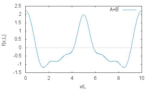
The ‘vector sum’   gives the expression

$$f_A(x;L) + f_B(x;L) = -{{\cos \left({{7\,\pi\,x}\over{5}}\right)}\over{7}}+{{\cos \left({{6\,\pi\,x}\over{5}}\right)}\over{6}}+{{13\,\cos \left({{4\,\pi\,x}\over{5}}\right)}\over{20}}+{{4\,\cos \left({{3\,\pi\,x}\over{5}}\right)}\over{15}}+{{13\,\cos \left({{2\,\pi\,x}\over{5}}\right)}\over{10}}$$

and the corresponding plot
fourier_vector_plot_A_plus_B

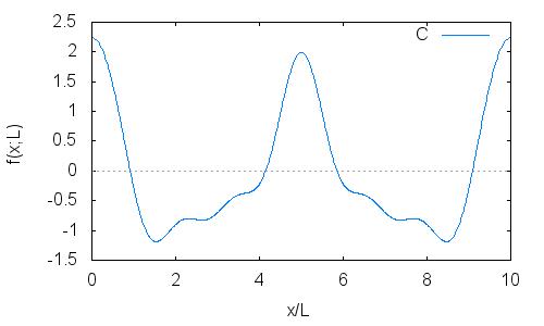
The student can then confirm this in terms of adding the list representations together by executing C = add_list(A,B) which yields

\[ C = \left[0,\frac{13}{10},\frac{4}{15},\frac{13}{20},0,\frac{1}{6},-\frac{1}{7}\right] \; .\]


Evaluating $$f_C(x;L)$$ = fourier_series(C;L) which yields the identical expression

$$f_C(x;L) = -{{\cos \left({{7\,\pi\,x}\over{5}}\right)}\over{7}}+{{\cos \left({{6\,\pi\,x}\over{5}}\right)}\over{6}}+{{13\,\cos \left({{4\,\pi\,x}\over{5}}\right)}\over{20}}+{{4\,\cos \left({{3\,\pi\,x}\over{5}}\right)}\over{15}}+{{13\,\cos \left({{2\,\pi\,x}\over{5}}\right)}\over{10}}$$

and the identical plot
fourier_vector_plot_C

Why Don’t We Teach the Helmholtz Theorem?

In an earlier post, I outlined a derivation of the Helmholtz Theorem starting from the identity

\[ \nabla^2 \left( \frac{1}{|\vec r – \vec r \, {}’|} \right) = -4 \pi \delta( \vec r – \vec r \, {}’ ) .\]

It seems hard for me to believe but it was many years after I had studied E&M in graduate school that I came across this theorem and to appreciate its power.  The reason I say it is hard for me to believe is that almost none of the traditional texts talk about it or even have an index entry for it.

The traditional way we teach electricity and magnetism is to trace through the historic development by examining a host of 18th and 19th century experiments. The usual course is to introduce integral forms of the laws and then show how these can lead to Maxwell’s equation (e.g., from Coulomb’s law to Gauss’s law).  The road here is long and tortuous, starting with static fields, then layering on the time dependence, and then finally sneaking the displacement current into Ampere’s law.  This approach obscures the unity of Maxwell’s equations.  It also leaves the student bored, confused, and overwhelmed, and incapable of appreciating what follows.

To such a student is lost the wonder of realizing that the fields can take on a life of their own, independent of the things that created them.  Lost is the realization that these fields can radiate outwards; that they can reflect and refract (i.e., optics as an inherently electromagnetic phenomenon); and that they can be generated and controlled at will to form the communication network we all use on a daily basis.

A better approach starts with Maxwell’s equations in their full form and then uses the Helmholtz theorem to ‘interrogate’ them to derive the time-honored static field results of Coulomb and Biot-Savart. I believe this approach, which is nearly impossible to find in the usual textbooks, offers a clearer view into the unity of electricity and magnetism, at the cost of some slightly more mature vector calculus.  The fields are introduced early, and the equations they satisfy are complete. There is no unlearning facts later on.  For example, the traditional textbook results for Coulomb’s law emphasize that the electric field is conservative and that its curl is identically zero.  Weeks or months go by with that concept firmly emphasized and entrenched and then, and only then, is the student informed that the result doesn’t hold in general.

There is also a fundamental flaw in the pedagogy of deriving Maxwell’s equations from the integral forms.  Nowhere along the line is there any explanation as to why knowing the divergence and curl of a vector field is all that is needed to uniquely specify the field. After all, why can’t a uniform field be added as a constant of integration?

At the heart of the traditional approach is the idea of a force field as a physically real object and not just a useful mathematical construct. The prototype example is the electric field, which comes from the experimental expression for Coulomb’s law, stating that the force on two charges $$q_2$$ due to $$q_1$$ is given by (note all equations are expressed in SI units):

\[ \vec F_{21}(\vec r) = \frac{1}{4 \pi \epsilon_0} \frac{ q_1 q_2 \left( \vec r_2 – \vec r_1 \right)}{|\vec r_2 – \vec r_1|^3} \, .\]

The usual practice is then to assume one of the charges is a test charge and that the other is smeared into an arbitrary charge distribution within a volume $$V$$ and that the resulting electric field is

\[ \vec E(\vec r) = \frac{1}{4 \pi \epsilon_0} \int_V d^3 r \frac{ \rho(\vec r \;’) \left( \vec r – \vec r \; ‘ \right)}{|\vec r – \vec r \; ‘|^3} \, . \]

The last step in the the traditional approach involves introducing vector field divergence and curl, the associated theorems they obey, and applying the whole lot to electric flux to get the first of the Maxwell equations

\[ \nabla \cdot \vec E (\vec r) = \rho(\vec r) / \epsilon_0 \, .\]

As the traditional program proceeds, magnetostatics follows with the introduction of the Biot-Savart law

\[ \vec B(\vec r) = \frac{\mu_0}{4 \pi} \int_V d^3 r’ \frac{ \vec J(\vec r \; ‘) \times (\vec r – \vec r \;’)}{|\vec r – \vec r \; ‘|^3} \, , \]

as the experimental observation for the generation of a magnetic field for a given current density within a volume $$V$$. This time the vanishing of the divergence is used to find the vector potential and the curl is related to the current density via Ampere’s law

\[ \nabla \times \vec B(\vec r) = \mu_0 \vec J(\vec r) \,.\]

The traditional approach finally gets to time-varying fields when taking up Faraday’s law, requiring the student to unlearn $$\nabla \times \vec E = 0$$ and then finally re-learn Ampere’s equation with the introduction of the displacement current. By this time the full Maxwell equations are on display, but the linkage between the different facets of each field is highly obscured, and the basic underpinning of the theory — that the divergence and curl tells all there is to know about a field — is not to be found. The pedagogy seems to suffer from too many unconnected facts with no common framework by which to relate them.

Using the Helmholtz Theorem in conjunction with an upfront statement of the Maxwell equations offers several advantages in teaching electromagnetism. I will content myself with just the derivation of the Coulomb’s and Biot-Savart’s law.  Additional information can be found in the paper and presentation I recently wrote for the Fall meeting of the Chesapeake Section of AAPT.

Start by considering the Maxwell equations, presented here in vacuum, as

\[ \nabla \cdot \vec E(\vec r,t) = \rho(\vec r,t) / \epsilon_0 \, ,\]

\[ \nabla \cdot \vec B(\vec r,t) = 0 \, , \]

\[ \nabla \times \vec E(\vec r,t) = -\frac{\partial \vec B (\vec r,t)}{\partial t} \, , \]

and

\[ \nabla \times \vec B(\vec r,t) = \mu_0 \vec J (\vec r,t) + \epsilon_0 \mu_0 \frac{\partial \vec E(\vec r,t)}{\partial t} \, .\]

Since the Coulomb and Biot-Savart laws are in the domain of the electro- and magnetostatics, all terms in Maxwell’s equations involving time derivatives are set equal to zero and all $$t$$’s are eliminated to yield
\[ \nabla \cdot \vec E(\vec r) = \rho(\vec r) / \epsilon_0 \, ,\]
\[ \nabla \cdot \vec B(\vec r) = 0 \, , \]
\[ \nabla \times \vec E(\vec r) = 0 \, , \]

and
\[ \nabla \times \vec B(\vec r) = \mu_0 \vec J (\vec r) \, .\]

Now substituting the electric and magnetic field divergences and curls into the $$U(\vec r)$$ and $$\vec W(\vec r)$$ expressions in Helmholtz’s theorem yields the usual scalar potential

\[U(\vec r) = \frac{1}{4 \pi \epsilon_0}\int_V d^3 r’ \frac{\rho(\vec r \;’)}{|\vec r – \vec r \;’|} \]

for the electric field and the usual vector potential

\[\vec W(\vec r) = \frac{\mu_0}{4\pi} \int_{V} d^3r’ \frac{ \vec J(\vec r) }{|\vec r – \vec r\;’|}\]

for the magnetic field.

On the whole, I think this approach enhances the physical understanding of Maxwell’s equations in ways the traditional approach can’t.  It’s not without its downside, but none of the problems present much difficulty.  Further details can be found in my paper.


Deriving the Helmholtz Theorem

To derive the Helmholtz theorem start first with one representation of the delta-function in 3-dimensions

\[ \nabla^2 \left( \frac{1}{|\vec r – \vec r \, {}’|} \right) = -4 \pi \delta( \vec r – \vec r \, {}’ ) \, .\]

Start with the identity
\[ \vec F(\vec r) = \int_{V} d^3 r’ \delta(\vec r – \vec r \,{}’) F(\vec r \,{}’) \]
for an arbitrary vector field $$\vec F(\vec r)$$ over a given volume $$V$$. Note that time will not be involved in this derivation. Also note that there is a ongoing discussion in the literature about the correct way to extend this theorem for time varying fields. This will be a discussed in a future post.

Using the explicit representation of the delta-function stated above and factoring out the derivatives with respect to the field point $$\vec r$$ yields

\[ \vec F(\vec r) = \frac{ -\nabla^2_{\vec r} }{4 \pi} \int_V d^3 r’ \frac{\vec F(\vec r\,{}’)}{|\vec r – \vec r\,{}’|} \, . \]

Now apply the vector identity $$\nabla^2 = \nabla( \nabla \cdot ) – \nabla \times (\nabla \times)$$. Doing so allows the expression for $$\vec F(\vec r)$$ to take the form
\[ \vec F (\vec r) = \frac{1}{4 \pi} \nabla_{\vec r} \times \vec I_{vector} – \frac{1}{4 \pi} \nabla_{\vec r} I_{scalar} \]
where the integrals
\[ \vec I_{vector} = \nabla_{\vec r} \times \int_v d^3 r ‘ \frac{\vec F (\vec r\,’)}{|\vec r – \vec r\,’|} \]
and
\[ I_{scalar} = \nabla_{\vec r} \cdot \int_v d^3 r ‘ \frac{\vec F (\vec r\,’)}{|\vec r – \vec r\,’|} \; . \]

The strategy for handling these terms is to

  1. bring the derivative operator with respect to r into the integral
  2. switch the derivative from r to r’ with a cost of a minus sign
  3. integrate by parts
  4. apply the appropriate boundary conditions and boundary integral version of the divergence theorem to the total derivative piece

Application of this strategy to the vector (first) integral gives
\[ \vec I _{vector} = \int_V d^3 r’ \frac{ \nabla_{\vec r\,’} \times \vec F (\vec r \, ‘)}{|\vec r – \vec r\,’|} – \int_{\partial V} dS \frac{\hat n \times \vec F(\vec r\,’)}{|\vec r – \vec r\,’|} \; .\]

Likewise, the same strategy applied to the scalar (second) integral gives
\[ I_{scalar} = \int_V d^3 r’ \frac{ \nabla \cdot \vec F ( \vec r \,’)}{|\vec r – \vec r\,’|} – \int_{\partial V} dS \frac{\hat n \cdot \vec F ( \vec r \,’)}{|\vec r – \vec r\,’|} \; . \]

Now the usual case of interest sets the bounding volume to be all space, which requires that the field drop off faster than $$r^{-1}$$. If this condition is met then the surface integrals zero and the original field can be written as
\[ \vec F (\vec r) = -\nabla U(\vec r) + \nabla \times \vec W(\vec r) \]
where
\[ U(\vec r) = \frac{1}{4\pi} \int_V d^3 r’ \frac{ \nabla’ \cdot \vec F ( \vec r \,’)}{|\vec r – \vec r\,’|} \]
and
\[ \vec W(\vec r) = \frac{1}{4\pi} \int_V d^3 r’ \frac{ \nabla’ \times \vec F ( \vec r \,’)}{|\vec r – \vec r\,’|} \; .\]

At this point it is a snap to derive Coulomb’s and Biot-Savart’s laws from the Maxwell equations but that is a post for another time.