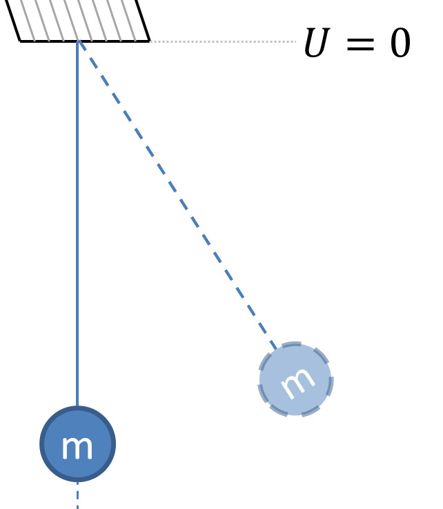
Numerical Solutions of the Pendulum
Last week’s column examined the use of the Lie series to the problem of the pendulum. As a model in classical mechanics, the pendulum is interesting since it is essentially nonlinear with a well-known analytic solution in terms of elliptic integrals. By essentially nonlinear, I mean that the problem doesn’t possess a nonlinear transformation that permits the differential equation to be recast as a linear problem, like is possible in the Kepler problem.
The comparison of the ‘exact’ solution in terms of elliptic integrals to the Lie series is very difficult. Expansions of the exact solution in power series in very complex due to both the Jacobi $$sn$$ function and the $$\sin^{-1}$$ in the analytic form. In contrast, the Lie series, which essentially generates the Taylor series in a compact, self-interative way, seems to not have any easily identified correspondence.
As a result, it seemed prudent to look at the numerical solutions of both approaches – exact and Lie series. Numerical integration using a Runge-Kutta integration scheme acts as a stand in for the exact elliptical integral solution. WxMaxima served as the tool to tackle this comparison as it does a fairly competent job of mixing symbolic and numerical processing (although it would be nice to try out a mix of numpy, scipy, and sympy in a Jupyter shell – perhaps sometime in the future).
To start, the $$D = \omega_0 \partial_{\theta_0} – g \sin(\theta_0) \partial_{\omega_0} $$ was defined as
D_pen(arg) := w*diff(arg,T) - g*sin(T)*diff(arg,w);
Two things are worth noting. First, the operator $$D$$ is given a decoration in the program so that, during testing, other functional forms could be used without clash. In particular, the use of $$D = \omega_0 \partial_{\theta_0} – g \theta_0 \partial_{\omega_0}$$ was especially helpful since the Lie expansion of the simple harmonic operator corresponds to the regular expansion of $$\sin$$ and $$\cos$$ and so is easy to check that the algorithm is correct. Second, note that the subscript reminding us that the operator acts upon the initial conditions has been suppressed. In some sense, it is not needed except as a reminder of that particular fact and, with that notion understood, it can be dropped.
The next order of business is to define a function that allows the formation of the Lie series based on $$D$$ to order $$n$$. This is accomplished using
L(order,D) := block([ret,temp],
                     ret  : T,
                     temp : T,
                     for n : 1 step 1 thru order do
                         block([],
                               temp : D(temp),
                               ret  : ret + t^n/n!*temp),
                     ret)$
As a test, L(4,D_pen) yields
\[ {{t^4\,\left(g^2\,\cos T\,\sin T+g\,w^2\,\sin T\right)}\over{24}}-{{g\,t^2\,\sin T}\over{2}}-{{g\,t^3\,w\,\cos T}\over{6}}+T+t\,w \; ,\]
which, up to a cosmetic change in notation, is seen to be the same expression as was derived last week.
The final function needed to complete the analysis is one that converts the symbolic form to numeric form for easy plotting and numerical comparisons. That function is defined as
Q(order,D,parms) := block([Lie],
                  Lie : L(order,D),
                  Lie : ev(Lie,parms));
What $$Q$$ does is to first retrieve the expression of the Lie series for a user-specified order and $$D$$ operator and then to evaluate that expression numerically using the $$ev$$ function built into Maxima. The list $$params$$ provides a convenient way to piggyback the appropriate parameters that match the problem at hand. These parameters include the numerical values of the initial conditions, any physical constants (e.g. $$g$$ in the problem of the pendulum), and the specific time at which the evaluation is to take place.
The next step is the solve the pendulum problem using a Runge Kutta and to assume that the resulting solution is close enough to the exact solution to be of use. The steps for this are fairly straightforward but a disciplined approach helps to remember the order of the arguments in the syntax.
The first step is to load the dynamics package using:
load("dynamics")
The second step is to define the physical constant for $$g$$
G : 10
(note that the symbol $$G$$ is chosen for the numerical value of $$g$$ to allow the later to stay as a symbolic quantity).
Next define the differential equations to be solved
dT_dt   : w;
dw_dt   : -G*sin(T);
my_odes : [dT_dt, dw_dt];
the names of the dynamic variables and their initial conditions
var_names : [T,w];
T0  : 2;
w0  : 0;
ICs : [T0,w0];
and the time mesh used for the integration
t_var   : t;
t_start : 0;
t_stop  : 3;
t_step  : 0.1;
t_domain: [t_var, t_start, t_stop, t_step];
Structured in this way, the call to the Runge Kutta integrator is nice and clean
Z : rk(my_odes, var_names, ICs, t_domain)$
The data structure $$Z$$ is a list of lists. Each of the sub-lists has three elements corresponding to the values of $$[t,\theta,\omega]$$ and the outside list has $$n$$ elements where $$n$$ is number of time points in the mesh defined above.
To make plots of the data requires massaging the results in a list of lists with only two elements (either $$[t,\theta]$$ or $$[t,\omega]$$) for use in a discrete plot. In addition, for proper comparison, similar lists are needed for the simple harmonic oscillator (as a linear problem baseline) and for different orders of the Lie series.
The built-in command makelist is the workhorse here with the desired list of lists being specified as
pen   : makelist( [Z[n][1],Z[n][2]],n,1,31)$
SHO   : makelist([(n-1)*0.1,2*cos(sqrt(10.0)*(n-1)*0.1)],n,1,31)$
Lie5  : makelist([(n-1)*0.1,Q(5,D_pen,[T=2.0,w=0.0,g=10.0,t=(n-1)*0.1])],n,1,31)$
Lie10 : makelist([(n-1)*0.1,Q(10,D_pen,[T=2.0,w=0.0,g=10.0,t=(n-1)*0.1])],n,1,31)$
These lists are then displayed using
wxplot2d([[discrete,pen],[discrete,SHO],[discrete,Lie5],[discrete,Lie10]],[x,0,1],[y,-2,2],[legend,"Pendulum","SHO","Lie5","Lie10"],[xlabel,"time"],[ylabel,"theta"]);
The resulting plot is
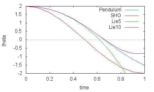
Several observations follow immediately from a careful inspection of this plot. First, the nonlinearity of the pendulum is quite obvious as the motion (blue trace) quickly departs from the corresponding motion from the simple harmonic oscillator (red trace). The Lie series capture this departure reasonable well as both the 5th and 10th order behavior (green and purple traces) sits on top of the exact solution for times less than 0.4. After this time, the 5th order begins diverging. The 10th order Lie series stays relatively close until a time of 0.7 where it too begins to diverge. Neither one makes it even a half a period, which is a disappointing observation. Clearly, while the Lie series is universal it is applicability it also seems to be universal in its limited range of convergence about the exact solution.