
For this go around with the Lie series, I thought it would be interesting to experiment with a problem quite unfamiliar to me – namely the full nonlinear pendulum equation. The approach here is two-fold. First, the classical computation for this key problem is presented. For this part, I use Lowenstein’s discussion in the book ‘Essentials of Hamiltonian Dynamics’ as a model. In the second part, I apply the Lie series to the system to see how well the generated expansion matches the classical result. The classical result requires a lot of familiarity with special functions and some clever and unmotivated substitutions. The hope here is that the brute force and straightforward method provided by the Lie series will be accurate enough when compared with the classical result to make it attractive.
Now to set the notation and conventions, consider the following figure of the pendulum.
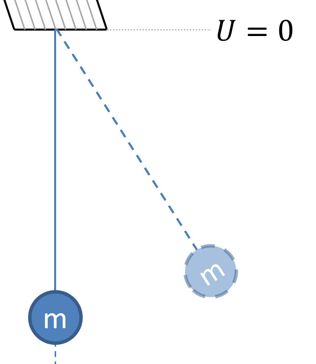
The angle $$\theta$$ from the vertical is clearly the only relevant degree of freedom. The pendulum bob of mass $$m$$ possesses a kinetic energy of
\[ K = \frac{1}{2} m R^2 \dot \theta^2 \; ,\]
where $$R$$ is the length of the pendulum. As denoted in the figure, the zero of the potential energy is taken when the bob is horizontal so that $$\theta = \frac{\pi}{2}$$. The potential energy function is then
\[ U = – m g R \cos \theta \; ,\]
For convenience in what follows, set $$m = 1$$ and $$R = 1$$. The Lagrangian of the system is then
\[ L(\theta,\dot \theta) = \frac{1}{2} \dot \theta ^2 + g \cos \theta \]
with the corresponding Euler-Lagrange equations of
\[ \ddot \theta + g \sin \theta = 0 \; .\]
The conjugate momentum
\[ p_{\theta} = \frac{\partial L}{\partial \dot \theta} = \dot \theta \]
becomes the new independent variable in the system when we switch to the Hamiltonian
\[ H(\theta,p_{\theta}) = \frac{p_{\theta}^2}{2} – g \cos \theta \; .\]
Since $$H(\theta,p_{\theta})$$ has no explicit time dependence,
\[ \frac{d H}{dt} = \frac{\partial H}{\partial t} = 0 \; ,\]
it is a conserved quantity that is the total energy.
With the conservation firmly in hand, we can eliminate the conjugate momentum in favor of the generalized velocity to get the energy equation
\[ \frac{1}{2} \dot \theta ^2 – g \cos \theta = E \; .\]
At this point, the special function gymnastics begin with the substitutions
\[ z = \frac{1}{k} sin \left( \frac{\theta}{2} \right) \]
and
\[ k = \sqrt{ \frac{E + g}{2 g} } \; ,\]
which bring the energy equation into the form
\[ \dot z ^2 = g(1-k^2 z^2) (1 – z^2) \; .\]
Solving this for $$dt$$ gives
\[ dt = \frac{dz}{ \sqrt{ g(1-k^2 z^2) (1 – z^2) } } \]
which integrates to
\[t – t_0 = \frac{1}{\sqrt{g}} \int_0^z \frac{d \zeta}{\sqrt{ g(1-k^2 \zeta^2) (1 – \zeta^2)}} \]
The integral on the right-hand side is important enough to have its own name – it is an elliptic integral of the first kind and its solutions are defined as
\[ F(sin^{-1} z|k^2) \equiv \frac{1}{\sqrt{g}} \int_0^z \frac{d \zeta}{\sqrt{ g(1-k^2 \zeta^2) (1 – \zeta^2) }}\]
By construction, $$k^2 \in [0,1)$$ corresponds to the librating situation where the bob has only enough energy to move to and fro without spinning about it point of rotation. The classical solution for $$z$$ is compactly written as
\[ z = sn(\sqrt{g}(t-t_0),k^2) \]
where $$sn$$ is the Jacobi elliptic integral. Inverting the defining relation between $$z$$ and $$\theta$$ gives the final solution as
\[ \theta(t) = 2 \sin^{-1}\left(k sn(\sqrt{g}t,k^2) \right) \; .\]
Understanding how to mine information from these expressions requires a fairly sophisticated understanding of the elliptical integrals, which, while important for this key problem, don’t translate universally.
To apply the Lie series, rewrite the equations of motion in state space form
\[ \frac{d}{dt} \left[ \begin{array}{c} \theta \\ \omega \end{array} \right] = \left[ \begin{array}{c} \omega \\ – g \sin \theta \end{array} \right] \]
from which is read the differential operator
\[ D = \omega_0 \partial_{\theta_0} – g \sin \theta_0 \partial_{\omega_0} \; .\]
The solution to the problem is then given by
\[ L[\theta_0] = e^{(t-t_0)D} \theta_0 \; .\]
As is usually the case, the Lie series is tractable to hand computations for the first few terms. The relevant operations with $$D$$ are:
\[ D \theta_0 = \omega_0 \; ,\]
\[ D^2 \theta_0 = – g \sin \theta_0 \; , \]
\[ D^3 \theta_0 = – g \omega_0 \cos \theta_0 \; , \]
and
\[ D^4 \theta_0 = g^2 \cos \theta_0 \sin \theta_0 + g \omega_0^2 \sin \theta_0 \; .\]
The resulting Lie series is quite unwieldy resulting in
\[ L[\theta_0] = \theta_0 – g \frac{(t-t_0)^2}{2!} \sin \theta_0 + \left( (t-t_0) – g \frac{(t-t_0)^3}{3!} \cos \theta_0 \right) \omega_0 \\ + \frac{(t-t_0)^4}{4!} \left( g^2 \cos \theta_0 \sin \theta_0 + g \omega_0^2 \sin \theta_0 \right) \; .\]
Unlike the Kepler case, the resulting Lie series for the pendulum doesn’t neatly separate into two pieces linear in the initial conditions. In addition, it isn’t at all clear how this expansion relates to the classical solution in terms of elliptic integrals. So it seems that in spite of its universal applicability, the Lie series is not a silver bullet.
Next week, I’ll take a look how closely the two approaches match numerically.