Monthly Archive: November 2015

I thought it might be nice to have a change of pace in this column and discuss some differential geometry and the relationship between classical vector analysis and the calculus of differential forms. In large measure, this dabbling is inspired by the article Differential forms as a basis for vector analysis – with applications to electrodynamics by Nathan Schleifer which appeared in the American Journal of Physics 51, 1139 (1983).

While I am not going to go into as much detail in this post as Schleifer did in his article, I do want to capture the flavor of what he was trying to do and set the groundwork for following posts on proving some of the many vector identities that he tackles (and perhaps a few that he doesn’t). At the botttom of all these endeavors is the pervading similarity of all of the various integral theorems of vector calculus.

The basis premise of the operation is to put into a one-to-one correspondence a classical vector expressed as

\[ \vec A = A_x \hat e_x + A_y \hat e_y + A_z \hat e_z \]

with an associated differential one-form

\[ \phi_{A} = A_x dx + A_y dy + A_z dz \; .\]

The elements of both descriptions form a vector space; that is to say that the 10 axioms of a vector space are satisfied by the objects in $$\{dx, dy, dz\}$$ just as they are satisfied by $$\{\hat e_x , \hat e_y, \hat e_z\}$$.

If decomposition into components were all that was required, the two notations would offer the same benefits with the only difference being the superficial differences in the glyphs of one set compared to another.

However, we want more out of our sets of objects. Exactly what additional structure each set caries and how it is notationally encoded is the major difference between the two approaches.

Typically, classical vectors are given a metric structure such that

\[ \hat e_i \cdot \hat e_j = \delta_{ij} \]

and a ‘cross’ structure such that

\[ \hat e_i \times \hat e_j = \epsilon_{ijk} e_k \; .\]

Differential one-forms differ in that they are given only the ‘cross’ structure in the form
\[ dy \wedge dz = – dz \wedge dy \; ,\]
\[ dz \wedge dx = – dx \wedge dz \; ,\]
\[ dx \wedge dy = – dy \wedge dx \; ,\]

where the wedge product $$dx \wedge dy$$ is sensibly called a two-form, indicating that it is made up of two one-forms.

Like the vector cross-product, the wedge product anti-commutes, implying that

\[ dx \wedge dx = 0 \; ,\]

with an analogous formula for $$dy$$ and $$dz$$.

Despite these similarities, the wedge product differs in one significant way from its vector cross-product cousin in that it is also associative so that no ambiguity exists by saying

\[ dx \wedge (dy \wedge dz) = (dx \wedge dy) \wedge dz = dx \wedge dy \wedge dz \; .\]

These algebraic rules are meant to sharply distinguish a point that is lost in classical vector analysis – namely that a vector defined in terms of a cross-product (i.e $$\vec C = \vec A \times \vec B$$) is not really a vector of the same type as the two vectors on the right-hand side that define it. That this must be true is easily (if somewhat startlingly) seen by the fact that when we consider the transformation of coordinates, the right-hand side needs two factors (one for $$\vec A$$ and one for $$\vec B$$) while the left-hand side needs only one. From a geometric point-of-view, we are exploiting a natural association between a plane spanned by $$\vec A$$ and $$\vec B$$ and the unique vector (up to a sign) that is perpendicular to it. This later obsservation is fully encoded into the structure of differential forms by defining the Hodge star operator such that

\[ dy \wedge dz \equiv *dx \; ,\]
\[ dz \wedge dx \equiv *dy \; ,\]
\[ dx \wedge dy \equiv *dz \; .\]

Also note that the Hodge star can be toggeled in the sense that

\[ *(dy \wedge dz) = **dx = dx \; ,\]

with similar expressions for the other two combinations.

Since the wedge product is associative, the Hodge star can be extended to operate on a three-form to give

\[ *(dx \wedge dy \wedge dz) = 1 \; , \]

which is interpreted as associating volumes with scalars.

All the tools are in place to follow the program of Schleifer for classical vector analysis. Note: some of these tools need to be modified for either higher dimensional spaces, or for non-positive-definite spaces, or both.

At this point, there may be some worry expressed that since the formalism of differential forms has no imposed metric structure, that we’ve thrown away the dot-product and all its useful properties. That this isn’t a problem can be seen as follows.

The classic dot-product is given by

\[ \vec A \cdot \vec B = A_x B_x + A_y B_y + A_z B_z \; .\]

The equivalent expression, in terms of forms, is

\[ \vec A \cdot \vec B \Leftrightarrow * ( \phi_{A} \wedge *\phi_B )\]

as can be seen as follows:

\[ \phi_B = B_x dx + B_y dy + B_z dz \; , \]

from which we get

\[ *\phi_B = B_x dy \wedge dz + B_y dz \wedge dx + B_z dx \wedge dy \; .\]

Now multiplying, from the left, by $$\phi_A$$ will lead to 9 products, each resulting in a three-form. However, due to the properties of the wedge product, only those products with a single $$dx$$, $$dy$$, and $$dz$$ will survive. These hardy terms are

\[ \phi_A \wedge *\phi_B = A_x B_x dx \wedge dy \wedge dz \\ + A_y B_y dy \wedge dz \wedge dx \\ + A_z B_z dz \wedge dx \wedge dy \; .\]

Accounting for the cyclic permutation of the wedge product this relation can be re-written as

\[ \phi_A \wedge *\phi_B = (A_x B_x + A_y B_y + A_z B_z) dx \wedge dy \wedge dz \; .\]

Applying the Hodge star operator immediately leads to

\[ * (\phi_A \wedge * \phi_B)) = A_x B_x + A_y B_y + A_z B_z \; . \]

In a similar fashion, the cross-product is seen to be
\[ \vec A \times \vec B \Leftrightarrow *(\phi_A \wedge \phi_B) \; .\]

The proof of this follows from

\[ \phi_A \wedge \phi_B = (A_x dx + A_y dy + A_z dz ) \wedge (B_x dx + B_y dy + B_z dz) \; ,\]

which expands to

\[ \phi_A \wedge \phi_B = (A_x B_y – A_y B_x) dx \wedge dy \\ + (A_y B_z – A_z B_y) dy \wedge dz \\ + (A_z B_x – A_x B_z) dz \wedge dx \; .\]

Applying the Hodge star operator gives

\[ *(\phi_A \wedge \phi_B) = (A_x B_y – A_y B_x) dz \\ + (A_y B_z – A_z B_y) dx \\ + (A_z B_x – A_x B_z) dy \equiv \phi_C \; ,\]

which gives an associated vector $$\vec C$$ of

\[ \phi_C \Leftrightarrow \vec C = (A_y B_z – A_z B_y) \hat e_x \\ + (A_z B_x – A_x B_z) \hat e_y \\ + (A_x B_y – A_y B_x) \hat e_z \; .\]

Next week, I’ll extend these results to include the classical vector analysis by use of the exterior derivative.

Change of pace is always good and, in this spirit, this week’s column will aims to model the solutions of the First-order Gauss Markov process. A First-order Gauss Markov process is a stochastic process that is used in certain applications for scheduling the injection of process noise into filtering methods. The basic idea is that during certain time periods, the internal physical process modelled in the filter will be insufficient due to the turning on and off of some additional, unmodelled force. Typical applications include the application of man-made controls to physical systems to force certain desirable behaviors.

The formulation of the First-order Gauss Markov process is usually done in terms of a stochastic equation. For simplicity, the scalar form will be studied. The generalization to the case with many components is straightforward and nothing is gained by the notational clutter. The equation we will analyze is
\[ {\dot x} = -\frac{1}{\tau} x + w \quad ,\]
where $$x(t)$$ is defined as the state and $$w$$ is a inhomogeneous noise term. In the absence of the noise, the solution is given by a trivial time integration to yield
\[ x_{h}(t) = x_{0} e^{ -(t-t_{0})/\tau } \quad , \]
assuming that $$x(t=t_{0}) = x_{0}$$. The solution $$x_h(t)$$ is known as the homogeneous solution and, as has often been discussed in this column, it will help in integrating the inhomogeneous term $$w$$. Ignore, for the moment, that $$w$$ (and, as a result, $$x$$) is a random variable. Treated as just an ordinary function, $$w$$ is a driving term that can be handled via the state transition matrix (essentially a one-sided Green’s function for an initial-value problem). Recall that a state transition matrix (STM) is defined as the object linking the state at time $$t_{0}$$ to the state at time $$t$$ according to
\[ x(t) = \Phi(t,t_{0}) x(t_{0}) \quad , \]
thus, by the definition, the STM is obtained as
\[ \Phi(t,t_{0}) = \frac{\partial x(t)}{\partial x(t_{0})} \quad . \]
Taking the partial derivative of homogeneous solution as required by the definition of the STM gives
\[ \Phi(t,t_{0}) = e^{ -(t-t_{0})/\tau } \quad . \]
The solution of the inhomogeneous equation is then given as
\[ x(t) = x_{h}(t) + \int_{t_{0}}^{t} \Phi(t,t’) w(t’) dt’ \quad .\]
As a check, take the time derivative of this expression to get
\[ {\dot x}(t) = {\dot x}_{h}(t) + \frac{d}{dt} \left[ \int_{t_{0}}^{t} \Phi(t,t’) w(t’) dt’ \right] \; \]
and then eliminate the time derivative on the two terms on the right-hand side by using the homogeneous differential equation for the first term and by using the Liebniz rule on the second term involving the integral
\[ {\dot x}(t) = -\frac{1}{\tau} x_{h}(t) + \Phi(t,t) w(t) + \int_{t_{0}}^{t} \frac{\partial \Phi(t,t’)}{\partial t} w(t’) dt’ \quad . \]
Since the following two conditions
\[ \Phi(t,t) = 1 \quad , \]
and
\[ \frac{\partial \Phi(t,t’)}{\partial t} = -\frac{1}{\tau} \Phi(t,t’) \quad , \]
are met, they can be substituted into the above expression. Doing so yields
\[ {\dot x}(t) = -\frac{1}{\tau} x_{h}(t) + w(t) – \frac{1}{\tau} \int_{t_{0}}^{t} \Phi(t,t’) w(t’) dt’ \; .\]
Grouping the terms in a suggestive way gives
\[ {\dot x}(t) = -\frac{1}{\tau} \left[ x_{h}(t) + \int_{t_{0}}^{t} \Phi(t,t’) w(t’) dt’ \right] + w(t) \; \]
from which immediately springs the recognition that
\[ {\dot x}(t) = -\frac{1}{\tau} x(t) + w(t) \quad \; , \]
which is what we were trying to prove.

It is worth noting that the condition listed for the time derivative of the STM is a specific example of the familiar form
\[ \frac{\partial \Phi(t,t’)}{\partial t} = A(t) \Phi(t,t’) \quad ,\]
where $$A(t)$$, known sometimes as the process matrix, is generally given by
\[ A(t) = \frac{\partial {\mathbf f}( {\mathbf x} (t) ) }{\partial {\mathbf x}(t)} \; .\]

With the general formalism well understood, the next step is to generate solutions. Since $$w(t)$$ is a noise term, each ensemble of realizations will birth a different response in $$x(t)$$ via the driving term in
\[ x(t) = x_{0} e^{ -(t-t_{0})/\tau } + \int_{t_{0}}^{t} e^{ -(t-t’)/\tau } w(t’) dt’ \; .\]
So there are an infinite number of solution and there is no practical way to deal with them as a group but statistically some meaningful statements can be made. The most useful statistical characterizations are found by computing the statistical moments about the origin (i.e. $$E[x^n(t)]$$, where $$E[\cdot]$$ denotes the expectation value of the argument).

In order to do this, we need to say something about the statistical distribution of the noise. We will assume that $$w(t)$$ is a Gaussian white-noise source with zero mean, a variance of $$q$$, and is uncorrelated. Mathematically these assertations amount to the condition $$E[w(t)] \equiv {\bar w} = 0$$ and the condition
\[ E[(w(t)-{\bar w}) (w(s) – {\bar w}) ] = E[ w(t)w(s) – {\bar w} w(t) – {\bar w} w(s) – {\bar w}^2 ] \\ = E[ w(t)w(s) ] = q \delta(t-s) \quad . \]

In addition, we assume that the state and the noise are statistically independent at different times
\[ E[x(t) w(s) ] = E[x(t)] E[w(s)] = 0 \quad . \]
Now we can compute the statistical moments of $$x(t)$$ about the origin.

The first moment is given by
\[ E[x(t)] = E \left[ x_{0} e^{ -(t-t_{0})/\tau } + \int_{t_{0}}^{t} e^{ -(t-t’)/\tau } w(t’) dt’ \right] \; .\]
Since the expectation operator is linear and since it only operates on $$x(t)$$ and $$w(t)$$ (they are the only two random variable) this expression becomes
\[ E[x(t)] = E \left[ x_{0} \right] e^{ -(t-t_{0})/\tau } + \int_{t_{0}}^{t} e^{ -(t-t’)/\tau } E \left[ w(t’) \right] dt’ \; .\]
From its statistical properties, $$E[w(t)] = $$ and so the above expression simplifies to
\[ E[x(t)] = E \left[ x_{0} \right] e^{ -(t-t_{0})/\tau } \; .\]

The second moment is more involved, although no more conceptually complicated, and is given by

\[ E[ x(t)^2 ] = E \left[ x_{0}^2 e^{ -2(t-t_{0})/\tau } \\ + 2 x_{0} e^{ -(t-t_{0})/\tau } \int_{t_{0}}^{t} e^{ -(t-t’)/\tau } w(t’) dt’ \\ + \int_{t_{0}}^{t} e^{ -(t-t’)/\tau } w(t’) dt’ \int_{t_{0}}^{t} e^{ -(t-t”)/\tau } w(t^{\prime\prime}) dt^{\prime\prime} \right] \; \]

Again using the facts that the expectation operator is linear and that the noise is zero mean, the second moment becomes

\[ E[x(t)] = E \left[x_{0}^2\right]e^{ -2(t-t_{0})/\tau } \\ + \int_{t_{0}}^{t} \int_{t_{0}}^{t} e^{ -(2t-t’-t”)/\tau } E \left[ w(t’) w(t^{\prime\prime}) \right] dt’ dt^{\prime\prime} \; .\]

Next we use the fact that the noise auto-correlation resolves to a delta function leaving behind

\[ E[x(t)] = E \left[x_{0}^2\right]e^{ -2(t-t_{0})/\tau } + \int_{t_{0}}^{t} \int_{t_{0}}^{t} e^{ -(2t-t’-t”)/\tau } + q \delta(t’-t”) dt’ dt^{\prime\prime} \; .\]

From there the final step is to use the properties of the delta-function to gid rid of one the integrals and then to explicitly evaluate the remaining one to get

\[ E[x(t)] = E \left[x_{0}^2\right]e^{ -2(t-t_{0})/\tau } + \frac{q \tau}{2} \left( 1 – e^{ -2(t-t_{0})/\tau } \right) \;.\]

With the first two moments in hand it is easy to get the variance

\[ E \left[x^2\right] – E\left[x\right]^2 = \left( E\left[x_{0}^2\right] – E \left[x_{0}\right]^2 \right) e^{-2(t-t_{0})/\tau} + \frac{q\tau}{2} \left(1- e^{-2(t-t_{0})/\tau} \right) \; ,\]

which can be re-written as

\[ {\mathcal P}(t) = {\mathcal P}_0 e^{ -2(t-t_0)/\tau } + \frac{q\tau}{2}\left(1-e^{-2(t-t_{0})/\tau}\right) \quad , \]

where $${\mathcal P_0} = \left( E\left[x_0^2\right] – E\left[x_0\right]^2 \right)$$ is the initial covariance.

The final step is to discuss exactly what these equations are telling. The solution for the mean suggests that the mean will, after a long time, settle in at a value of zero regardless of the initial conditions for $$x_0$$. The variance equation then tells us that the uncertainty or dispersion about this zero-mean grows as $$\sqrt{t}$$ (since the only long-time term in the variance is proportional to $$t$$). This behavior is suggestive of a random walk. One of the more useful applications of this formalism to schedule in the parameter $$q$$ and being non-zero only within a certain time span. During this time span, the variance of process ‘opens up’ thereby allowing more freedom for a filter to heed measurement data rather than paying strict attention to its internal process. Thus a First-order Gauss Markov process, when scheduled into an underlying physical process, allows for modern filters to tracking unmodeled forces.

Last week I covered some nice properties associated with the looking at a matrix in terms of its rows and its columns as entities in their own sense. This week, I thought would put some finishing touches on these points with a few additional items to clean up the corners, as it were.

Transforming Coordinates

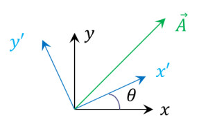
The biggest reason, or perhaps clue, for regarding row and/or columns of matrices as having an identity apart from the matrix itself comes from the general theory of changing coordinates. We start in two dimensions (the generalization to $$N$$ dimensions is obvious) with an arbitrary vector $$\vec A$$ and two different coordinate systems $${\mathcal O}$$ and $${\mathcal O}’$$ being used in its description. The relevant geometry is shown below.

We can consider the two frames as being spanned by the set of orthogonal vectors $$\{\hat e_x, \hat e_y\}$$ and $$\{\hat e_{x’}, \hat e_{y’}\}$$, respectively. Now the obvious decomposition of the vector is both frames leads to

\[ \vec A = A_x \hat e_x + A_y \hat e_y \]

and

\[ \vec A = A_{x’} \hat e_{x’} + A_{y’} \hat e_{y’} \; .\]

The fun begins when we note that the individual components of $$\vec A$$ are obtained by taking the appropriate dot-products between it and the basis vectors. It is straightforward to see that

\[ A_x = \vec A \cdot \hat e_x \]

since

\[ \vec A \cdot \hat e_x = \left(A_x \hat e_x + A_y \hat e_y \right) \cdot \hat e_x = A_x \hat e_x \cdot \hat e_x + A_y \hat e_y \cdot \hat e_x = A_x \; .\]

The last relation follows from the mutual orthogonality of the basis vectors, which is summarized as

\[ \hat e_i \cdot \hat e_j = \delta_{ij} \; ,\]

where $$\delta_{ij}$$ is the usual Kronecker delta.

The fun builds when we allow $$\vec A$$ to be expressed in the alternate frame from the one whose basis vector is being used in the dot-product. This ‘mixed’ dot-product serves as the bridge needed to cross between the two frames as follows.

\[ \vec A \cdot \hat e_x = \left( A_{x’} \hat e_{x’} + A_{y’} \hat e_{y’} \right) \cdot \hat e_x \; .\]

On one hand, $$\vec A \cdot \hat e_x = A_x$$, as was established above. On the other, it takes the form

\[\vec A \cdot \hat e_{x’} = A_{x’} \hat e_{x’} \cdot \hat e_{x} + A_{y’} \hat e_{y’} \cdot \hat e_{x} \; .\]

Equating the two expressions gives the ‘bridge relation’ between the two frames. Carrying this out for the other components leads to the matrix relation between the components in different frames given by

\[ \left[ \begin{array}{c} A_{x’} \\ A_{y’} \end{array} \right] = \left[ \begin{array}{cc}\hat e_{x’} \cdot \hat e_{x} & \hat e_{x’} \cdot \hat e_y \\ \hat e_{y’} \cdot \hat e_{x} & \hat e_{y’} \cdot \hat e_y \end{array} \right] \left[ \begin{array}{c} A_x \\ A_y \end{array} \right] \; .\]

A bit of reflection should allow on to see that the rows of the $$2 \times 2$$ matrix that connects the right-hand side to the left are the components of $$\hat e_{x’}$$ and $$\hat e_{y’}$$ expressed in the $${\mathcal O}$$ frame. Likewise, the columns of the same matrix are the components of $$\hat e_x$$ and $$\hat e_y$$ expressed in the $${\mathcal O}’$$ frame. Since there is nothing special about which frame is really labelled $${\mathcal O}$$ and which is labelled $${\mathcal O}’$$, it follows logically that the transpose of the matrix must be its own inverse. Therefore, we’ve arrived at the concept of an orthogonal matrix.

Units

Following hard on the heels of the previous result is a comment on the units born by the elements of a matrix. While mathematics likes to have pure numbers, the practicing physical scientist is not afforded that luxury. If we regard an arbitrary matrix has having units (that is each element has the same units) then the column arrays $$|e_i\rangle$$ must also have the same units. But the row arrays $$\langle \omega_j|$$ must have the inverse units for two very good reasons.

First the relations $$\langle \omega_j | e_i \rangle = \delta_{ij}$$ and the $$\sum_i |e_i\rangle \langle \omega_i| = {\mathbf Id}$$ (where $${\mathbf Id}$$ is the $$N \times N$$ identity matrix) demand that the rows have inverse units compared to the columns. Second, the determinant of the original matrix has units of the original base raised to the $$N$$-th power for a $$N \times N$$ matrix. Classical matrix inverse theory requires that the components of the inverse are proportional to the determinant of some $$N-1 \times N-1$$ minor of the same matrix divided by the determinant. The net effect being that those components of the inverse matrix have inverse coefficients.

In the change of coordinates, the fact that the basis vectors are unitless is exactly the explanation why a transpose can be an inverse. The fact that the student is usually exposed to matrices first in the context of the change in coordinates actually leads to a lot of confusion that could be avoided by first starting with matrices that have units.

Diagonalizing a Matrix

Finally, there is often some confusion surrounding the connection between vectors and diagonalizing a matrix. Specifically, beginners are often daunted by what appears to be the mysterious connection between the eigenvector/eigenvalue relation

\[ {\mathbf M} \vec e_i = \lambda_i \vec e_i \; .\]

With the division of a matrix into row- and column arrays the connection becomes much clearer. It starts with the hypothesis that there exists a matrix $${\mathbf S}$$ such that

\[ {\mathbf S}^{-1} {\mathbf M} {\mathbf S} = diag(\lambda_1, \lambda_2, \ldots, \lambda_N) \; , \]

where $$diag(\lambda_1, \lambda_2, \ldots, \lambda_N)$$ is a diagonal matrix of the same size as $${\mathbf M}$$. Note that this form ignores the complication of degeneracy but it is not essential since the Gram-Schmidt method can be used to further diagonalize the degenerate subspaces.

We then divide $${\mathbf S}$$ and its inverse as

\[ {\mathbf S} = \left[ \begin{array}{cccc} |e_1\rangle & |e_2\rangle & \ldots & |e_N\rangle \end{array} \right] \]

and

\[ {\mathbf S}^{-1} = \left[ \begin{array}{c} \langle \omega_1 | \\ \langle \omega_2 | \\ \vdots \\ \langle \omega_N| \end{array} \right] \; .\]

The hypothesis is then confirmed if there are $$|e_i\rangle$$ that are eigenvectors of $${\mathbf M}$$ since

\[ {\mathbf M}{\mathbf S} ={\mathbf M} \left[ \begin{array}{cccc} |e_1\rangle & |e_2\rangle & \ldots & |e_N\rangle \end{array} \right] = \left[ \begin{array}{cccc} \lambda_1 |e_1\rangle & \lambda_2 |e_2\rangle & \ldots & \lambda_N |e_N\rangle \end{array} \right] \; .\]

It then follows that

\[ {\mathbf S}^{-1} {\mathbf M}{\mathbf S} = \left[ \begin{array}{c} \langle \omega_1 | \\ \langle \omega_2 | \\ \vdots \\ \langle \omega_N| \end{array} \right] \left[ \begin{array}{cccc} \lambda_1 |e_1\rangle & \lambda_2 |e_2\rangle & \ldots & \lambda_N |e_N\rangle \end{array} \right] \\ = \left[ \begin{array}{cccc} \lambda_1 \langle \omega_1 | e_1\rangle & \lambda_2 \langle \omega_1 | e_2\rangle & \ldots & \lambda_1 \langle \omega_1 | e_N\rangle \\ \vdots & \vdots & \ddots & \vdots \\ \lambda_N \langle \omega_N | e_1\rangle & \lambda_N \langle \omega_N | e_2\rangle & \ldots & \lambda_N \langle \omega_N | e_N\rangle \end{array} \right] \; .\]

Using the basic relationship between the row- and column arrays, the above equation simplifies to

\[ {\mathbf S}^{-1} {\mathbf M}{\mathbf S} = \left[ \begin{array}{cccc} \lambda_1 & 0 & \ldots & 0 \\ \vdots & \vdots & \ddots & \vdots \\ 0 & 0 & \ldots & \lambda_N \end{array} \right] \; .\]

This approach is nice, clean, economical, and it stresses when the special cases with orthogonal (or unitary, or whatever) matrices apply.

One of the most ubiquitous tools in the physical scientists toolbox is the use of linear algebra for organizing systems with multiple degrees of freedom. Since it is ubiquitous it is hardly a surprise that there are almost as many notations as there are authors. I suppose what I am about to present is peculiar to my way of thinking but I find it both insightful and appealing.

Take a matrix $$\mathbf{M}$$ and segregate it into column arrays labeled as $$|e_i\rangle$$ defined by:

\[ \mathbf{M} = \left[ \begin{array}{cccc} |e_1\rangle & |e_2\rangle & \ldots & |e_n\rangle \end{array} \right] \; \]

The use of the Dirac notation to specify the column arrays that comprise the original matrix is intentional.

Likewise segregate the inverse matrix, whose relationship to the original matrix is yet to be determined, into row arrays labeled as $$\langle \omega_j|$$ defined by:

\[ \mathbf{M}^{-1} = \left[ \begin{array}{c} \langle\omega_1| \\ \langle\omega_2| \\ \vdots \\ \langle\omega_n| \end{array} \right] \]

Since we will demand that the matrix inverse left-multiplying the matrix must be the identity

\[ \mathbf{M}^{-1} \mathbf{M} = \left[ \begin{array}{c} \langle\omega_1| \\ \langle\omega_2| \\ \vdots \\ \langle\omega_n| \end{array} \right] \left[ \begin{array}{cccc} |e_1\rangle & |e_2\rangle & \ldots & |e_n\rangle \end{array} \right] \; .\]

This particular product is between a $$N \times 1$$ matrix of row arrays and $$1 \times N$$ matrix of column arrays. Since the $$\langle \omega_j$$ are $$1 \times N$$ matrices and the $$| e_i \rangle$$ are $$N \times 1$$ and the subsequent products are $$ 1 \times 1 $$ arrays (i.e. numbers) arranged as $$N \times N $$ matrix.

\[ \mathbf{M}^{-1} \mathbf{M} = \left[ \begin{array}{cccc} \langle\omega_1|e_1\rangle & \langle\omega_1|e_2\rangle & \ldots & \langle\omega_1|e_n\rangle \\ \langle\omega_2|e_1\rangle & \langle\omega_2|e_2\rangle & \ldots & \langle\omega_2|e_n\rangle \\ \vdots & \vdots & \ddots & \vdots \\ \langle\omega_n|e_1\rangle & \langle\omega_n|e_2\rangle & \ldots & \langle\omega_n|e_n\rangle \end{array} \right] \]

In order for this matrix to be the identity the following relation

\[ \langle\omega_i|e_j\rangle = \delta_{ij} \]

must hold.

In an analogous fashion, the left-multiplication of the inverse by the original matrix gives
\[ \mathbf{M} \mathbf{M}^{-1} = \left[ \begin{array}{cccc} |e_1\rangle & |e_2\rangle & \ldots & |e_n\rangle \end{array} \right] \left[ \begin{array}{c} \langle\omega_1| \\ \langle\omega_2| \\ \vdots \\ \langle\omega_n| \end{array} \right] \; .\]

This particular product is between $$1 \times N$$ matrix of column arrays and $$N \times 1$$ matrix of row arrays. This leads to a $$1 \times 1$$ sum of outer products

\[ \mathbf{M} \mathbf{M}^{-1} = \sum_i |e_i\rangle\langle\omega_i| \; . \]

Setting this sum to the identity gives

\[ \sum_i |e_i\rangle\langle\omega_i| = \mathbf{Id} \; .\]

This formalism is most easy to understand when the matrix is a $$2 \times 2$$ matrix of the form

\[ \mathbf{M} = \left[ \begin{array}{cc} a & b \\ c & d \end{array} \right] \; .\]

The well known inverse is

\[ \mathbf{M}^{-1} = \frac{1}{ad-bc} \left[ \begin{array}{cc} d & -b \\ -c & a \end{array} \right] \equiv q \left[ \begin{array}{cc} d & -b \\ -c & a \end{array} \right] \; .\]

From these forms, it is easy to read off

\[ |e_1\rangle = \left[ \begin{array}{c} a \\c \end{array} \right] \; ,\]

\[ |e_2\rangle = \left[ \begin{array}{c} b \\d \end{array} \right] \; ,\]

\[ \langle \omega_1| = q \left[ \begin{array}{cc} d & -b \end{array} \right] \; , \]

and

\[ \langle \omega_2| = q \left[ \begin{array}{cc} -c & a \end{array} \right] \; ,\]

where $$q = a d – b c$$, which is the determinant of $$\mathbf{M}$$.

Working the matrix elements resulting from $$\mathbf{M}^{-1} \mathbf{M}$$, it is easy to see that
\[ \langle \omega_1 | e_1 \rangle = q \left[ \begin{array}{cc} d & -b \end{array} \right] \left[ \begin{array}{c} a \\c \end{array} \right] = q (ad-bc) = \frac{ad-bc}{ad-bc} = 1 \; , \]

\[ \langle \omega_1 | e_2 \rangle = q \left[ \begin{array}{cc} d & -b \end{array} \right] \left[ \begin{array}{c} b \\d \end{array} \right] = q (db-bd) = 0 \; ,\]

\[ \langle \omega_2 | e_1 \rangle = q \left[ \begin{array}{cc} -c & a \end{array} \right] \left[ \begin{array}{c} a \\c \end{array} \right] = q (-ca + ac) = 0 \; ,\]

and

\[ \langle \omega_2 | e_2 \rangle = q \left[ \begin{array}{cc} -c & a \end{array} \right] \left[ \begin{array}{c} b \\d \end{array} \right] = q (-cb + ad) = \frac{ad-bc}{ad-bc} = 1 \; .\]

Working the outer products resulting from $$\mathbf{M} \mathbf{M}^{-1}$$, it is also easy to see that
\[ | e_1 \rangle \langle \omega_1 | = q \left[ \begin{array}{c} a \\c \end{array} \right] \left[ \begin{array}{cc} d & -b \end{array} \right] = q \left[ \begin{array}{cc} a d & -a b \\ c d & -c b \end{array} \right]\]

and

\[ | e_2 \rangle \langle \omega_2 | = q \left[ \begin{array}{c} b \\d \end{array} \right] \left[ \begin{array}{cc} -c & a \end{array} \right] = q \left[ \begin{array}{cc} -b c & b a \\ -c d & a d \end{array} \right] \; .\]

Summing these two matrices gives

\[ | e_1 \rangle \langle \omega_1 | + | e_2 \rangle \langle \omega_2 | = q \left[ \begin{array}{cc} ad-bc & -ab + ab \\ cd – cd & a d – b c \end{array} \right] = \left[ \begin{array}{cc} 1 & 0 \\ 0 & 1 \end{array} \right] \; .\]

It all works, as if by magic, but it is simply a result of some reasonably well-structured definitions.