
Last week I covered some nice properties associated with the looking at a matrix in terms of its rows and its columns as entities in their own sense. This week, I thought would put some finishing touches on these points with a few additional items to clean up the corners, as it were.
Transforming Coordinates
The biggest reason, or perhaps clue, for regarding row and/or columns of matrices as having an identity apart from the matrix itself comes from the general theory of changing coordinates. We start in two dimensions (the generalization to $$N$$ dimensions is obvious) with an arbitrary vector $$\vec A$$ and two different coordinate systems $${\mathcal O}$$ and $${\mathcal O}’$$ being used in its description. The relevant geometry is shown below.
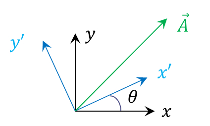
We can consider the two frames as being spanned by the set of orthogonal vectors $$\{\hat e_x, \hat e_y\}$$ and $$\{\hat e_{x’}, \hat e_{y’}\}$$, respectively. Now the obvious decomposition of the vector is both frames leads to
\[ \vec A = A_x \hat e_x + A_y \hat e_y \]
and
\[ \vec A = A_{x’} \hat e_{x’} + A_{y’} \hat e_{y’} \; .\]
The fun begins when we note that the individual components of $$\vec A$$ are obtained by taking the appropriate dot-products between it and the basis vectors. It is straightforward to see that
\[ A_x = \vec A \cdot \hat e_x \]
since
\[ \vec A \cdot \hat e_x = \left(A_x \hat e_x + A_y \hat e_y \right) \cdot \hat e_x = A_x \hat e_x \cdot \hat e_x + A_y \hat e_y \cdot \hat e_x = A_x \; .\]
The last relation follows from the mutual orthogonality of the basis vectors, which is summarized as
\[ \hat e_i \cdot \hat e_j = \delta_{ij} \; ,\]
where $$\delta_{ij}$$ is the usual Kronecker delta.
The fun builds when we allow $$\vec A$$ to be expressed in the alternate frame from the one whose basis vector is being used in the dot-product. This ‘mixed’ dot-product serves as the bridge needed to cross between the two frames as follows.
\[ \vec A \cdot \hat e_x = \left( A_{x’} \hat e_{x’} + A_{y’} \hat e_{y’} \right) \cdot \hat e_x \; .\]
On one hand, $$\vec A \cdot \hat e_x = A_x$$, as was established above. On the other, it takes the form
\[\vec A \cdot \hat e_{x’} = A_{x’} \hat e_{x’} \cdot \hat e_{x} + A_{y’} \hat e_{y’} \cdot \hat e_{x} \; .\]
Equating the two expressions gives the ‘bridge relation’ between the two frames. Carrying this out for the other components leads to the matrix relation between the components in different frames given by
\[ \left[ \begin{array}{c} A_{x’} \\ A_{y’} \end{array} \right] = \left[ \begin{array}{cc}\hat e_{x’} \cdot \hat e_{x} & \hat e_{x’} \cdot \hat e_y \\ \hat e_{y’} \cdot \hat e_{x} & \hat e_{y’} \cdot \hat e_y \end{array} \right] \left[ \begin{array}{c} A_x \\ A_y \end{array} \right] \; .\]
A bit of reflection should allow on to see that the rows of the $$2 \times 2$$ matrix that connects the right-hand side to the left are the components of $$\hat e_{x’}$$ and $$\hat e_{y’}$$ expressed in the $${\mathcal O}$$ frame. Likewise, the columns of the same matrix are the components of $$\hat e_x$$ and $$\hat e_y$$ expressed in the $${\mathcal O}’$$ frame. Since there is nothing special about which frame is really labelled $${\mathcal O}$$ and which is labelled $${\mathcal O}’$$, it follows logically that the transpose of the matrix must be its own inverse. Therefore, we’ve arrived at the concept of an orthogonal matrix.
Units
Following hard on the heels of the previous result is a comment on the units born by the elements of a matrix. While mathematics likes to have pure numbers, the practicing physical scientist is not afforded that luxury. If we regard an arbitrary matrix has having units (that is each element has the same units) then the column arrays $$|e_i\rangle$$ must also have the same units. But the row arrays $$\langle \omega_j|$$ must have the inverse units for two very good reasons.
First the relations $$\langle \omega_j | e_i \rangle = \delta_{ij}$$ and the $$\sum_i |e_i\rangle \langle \omega_i| = {\mathbf Id}$$ (where $${\mathbf Id}$$ is the $$N \times N$$ identity matrix) demand that the rows have inverse units compared to the columns. Second, the determinant of the original matrix has units of the original base raised to the $$N$$-th power for a $$N \times N$$ matrix. Classical matrix inverse theory requires that the components of the inverse are proportional to the determinant of some $$N-1 \times N-1$$ minor of the same matrix divided by the determinant. The net effect being that those components of the inverse matrix have inverse coefficients.
In the change of coordinates, the fact that the basis vectors are unitless is exactly the explanation why a transpose can be an inverse. The fact that the student is usually exposed to matrices first in the context of the change in coordinates actually leads to a lot of confusion that could be avoided by first starting with matrices that have units.
Diagonalizing a Matrix
Finally, there is often some confusion surrounding the connection between vectors and diagonalizing a matrix. Specifically, beginners are often daunted by what appears to be the mysterious connection between the eigenvector/eigenvalue relation
\[ {\mathbf M} \vec e_i = \lambda_i \vec e_i \; .\]
With the division of a matrix into row- and column arrays the connection becomes much clearer. It starts with the hypothesis that there exists a matrix $${\mathbf S}$$ such that
\[ {\mathbf S}^{-1} {\mathbf M} {\mathbf S} = diag(\lambda_1, \lambda_2, \ldots, \lambda_N) \; , \]
where $$diag(\lambda_1, \lambda_2, \ldots, \lambda_N)$$ is a diagonal matrix of the same size as $${\mathbf M}$$. Note that this form ignores the complication of degeneracy but it is not essential since the Gram-Schmidt method can be used to further diagonalize the degenerate subspaces.
We then divide $${\mathbf S}$$ and its inverse as
\[ {\mathbf S} = \left[ \begin{array}{cccc} |e_1\rangle & |e_2\rangle & \ldots & |e_N\rangle \end{array} \right] \]
and
\[ {\mathbf S}^{-1} = \left[ \begin{array}{c} \langle \omega_1 | \\ \langle \omega_2 | \\ \vdots \\ \langle \omega_N| \end{array} \right] \; .\]
The hypothesis is then confirmed if there are $$|e_i\rangle$$ that are eigenvectors of $${\mathbf M}$$ since
\[ {\mathbf M}{\mathbf S} ={\mathbf M} \left[ \begin{array}{cccc} |e_1\rangle & |e_2\rangle & \ldots & |e_N\rangle \end{array} \right] = \left[ \begin{array}{cccc} \lambda_1 |e_1\rangle & \lambda_2 |e_2\rangle & \ldots & \lambda_N |e_N\rangle \end{array} \right] \; .\]
It then follows that
\[ {\mathbf S}^{-1} {\mathbf M}{\mathbf S} = \left[ \begin{array}{c} \langle \omega_1 | \\ \langle \omega_2 | \\ \vdots \\ \langle \omega_N| \end{array} \right] \left[ \begin{array}{cccc} \lambda_1 |e_1\rangle & \lambda_2 |e_2\rangle & \ldots & \lambda_N |e_N\rangle \end{array} \right] \\ = \left[ \begin{array}{cccc} \lambda_1 \langle \omega_1 | e_1\rangle & \lambda_2 \langle \omega_1 | e_2\rangle & \ldots & \lambda_1 \langle \omega_1 | e_N\rangle \\ \vdots & \vdots & \ddots & \vdots \\ \lambda_N \langle \omega_N | e_1\rangle & \lambda_N \langle \omega_N | e_2\rangle & \ldots & \lambda_N \langle \omega_N | e_N\rangle \end{array} \right] \; .\]
Using the basic relationship between the row- and column arrays, the above equation simplifies to
\[ {\mathbf S}^{-1} {\mathbf M}{\mathbf S} = \left[ \begin{array}{cccc} \lambda_1 & 0 & \ldots & 0 \\ \vdots & \vdots & \ddots & \vdots \\ 0 & 0 & \ldots & \lambda_N \end{array} \right] \; .\]
This approach is nice, clean, economical, and it stresses when the special cases with orthogonal (or unitary, or whatever) matrices apply.