One of the most ubiquitous tools in the physical scientists toolbox is the use of linear algebra for organizing systems with multiple degrees of freedom. Since it is ubiquitous it is hardly a surprise that there are almost as many notations as there are authors. I suppose what I am about to present is peculiar to my way of thinking but I find it both insightful and appealing.

Take a matrix $$\mathbf{M}$$ and segregate it into column arrays labeled as $$|e_i\rangle$$ defined by:

\[ \mathbf{M} = \left[ \begin{array}{cccc} |e_1\rangle & |e_2\rangle & \ldots & |e_n\rangle \end{array} \right] \; \]

The use of the Dirac notation to specify the column arrays that comprise the original matrix is intentional.

Likewise segregate the inverse matrix, whose relationship to the original matrix is yet to be determined, into row arrays labeled as $$\langle \omega_j|$$ defined by:

\[ \mathbf{M}^{-1} = \left[ \begin{array}{c} \langle\omega_1| \\ \langle\omega_2| \\ \vdots \\ \langle\omega_n| \end{array} \right] \]

Since we will demand that the matrix inverse left-multiplying the matrix must be the identity

\[ \mathbf{M}^{-1} \mathbf{M} = \left[ \begin{array}{c} \langle\omega_1| \\ \langle\omega_2| \\ \vdots \\ \langle\omega_n| \end{array} \right] \left[ \begin{array}{cccc} |e_1\rangle & |e_2\rangle & \ldots & |e_n\rangle \end{array} \right] \; .\]

This particular product is between a $$N \times 1$$ matrix of row arrays and $$1 \times N$$ matrix of column arrays. Since the $$\langle \omega_j$$ are $$1 \times N$$ matrices and the $$| e_i \rangle$$ are $$N \times 1$$ and the subsequent products are $$ 1 \times 1 $$ arrays (i.e. numbers) arranged as $$N \times N $$ matrix.

\[ \mathbf{M}^{-1} \mathbf{M} = \left[ \begin{array}{cccc} \langle\omega_1|e_1\rangle & \langle\omega_1|e_2\rangle & \ldots & \langle\omega_1|e_n\rangle \\ \langle\omega_2|e_1\rangle & \langle\omega_2|e_2\rangle & \ldots & \langle\omega_2|e_n\rangle \\ \vdots & \vdots & \ddots & \vdots \\ \langle\omega_n|e_1\rangle & \langle\omega_n|e_2\rangle & \ldots & \langle\omega_n|e_n\rangle \end{array} \right] \]

In order for this matrix to be the identity the following relation

\[ \langle\omega_i|e_j\rangle = \delta_{ij} \]

must hold.

In an analogous fashion, the left-multiplication of the inverse by the original matrix gives
\[ \mathbf{M} \mathbf{M}^{-1} = \left[ \begin{array}{cccc} |e_1\rangle & |e_2\rangle & \ldots & |e_n\rangle \end{array} \right] \left[ \begin{array}{c} \langle\omega_1| \\ \langle\omega_2| \\ \vdots \\ \langle\omega_n| \end{array} \right] \; .\]

This particular product is between $$1 \times N$$ matrix of column arrays and $$N \times 1$$ matrix of row arrays. This leads to a $$1 \times 1$$ sum of outer products

\[ \mathbf{M} \mathbf{M}^{-1} = \sum_i |e_i\rangle\langle\omega_i| \; . \]

Setting this sum to the identity gives

\[ \sum_i |e_i\rangle\langle\omega_i| = \mathbf{Id} \; .\]

This formalism is most easy to understand when the matrix is a $$2 \times 2$$ matrix of the form

\[ \mathbf{M} = \left[ \begin{array}{cc} a & b \\ c & d \end{array} \right] \; .\]

The well known inverse is

\[ \mathbf{M}^{-1} = \frac{1}{ad-bc} \left[ \begin{array}{cc} d & -b \\ -c & a \end{array} \right] \equiv q \left[ \begin{array}{cc} d & -b \\ -c & a \end{array} \right] \; .\]

From these forms, it is easy to read off

\[ |e_1\rangle = \left[ \begin{array}{c} a \\c \end{array} \right] \; ,\]

\[ |e_2\rangle = \left[ \begin{array}{c} b \\d \end{array} \right] \; ,\]

\[ \langle \omega_1| = q \left[ \begin{array}{cc} d & -b \end{array} \right] \; , \]

and

\[ \langle \omega_2| = q \left[ \begin{array}{cc} -c & a \end{array} \right] \; ,\]

where $$q = a d – b c$$, which is the determinant of $$\mathbf{M}$$.

Working the matrix elements resulting from $$\mathbf{M}^{-1} \mathbf{M}$$, it is easy to see that
\[ \langle \omega_1 | e_1 \rangle = q \left[ \begin{array}{cc} d & -b \end{array} \right] \left[ \begin{array}{c} a \\c \end{array} \right] = q (ad-bc) = \frac{ad-bc}{ad-bc} = 1 \; , \]

\[ \langle \omega_1 | e_2 \rangle = q \left[ \begin{array}{cc} d & -b \end{array} \right] \left[ \begin{array}{c} b \\d \end{array} \right] = q (db-bd) = 0 \; ,\]

\[ \langle \omega_2 | e_1 \rangle = q \left[ \begin{array}{cc} -c & a \end{array} \right] \left[ \begin{array}{c} a \\c \end{array} \right] = q (-ca + ac) = 0 \; ,\]

and

\[ \langle \omega_2 | e_2 \rangle = q \left[ \begin{array}{cc} -c & a \end{array} \right] \left[ \begin{array}{c} b \\d \end{array} \right] = q (-cb + ad) = \frac{ad-bc}{ad-bc} = 1 \; .\]

Working the outer products resulting from $$\mathbf{M} \mathbf{M}^{-1}$$, it is also easy to see that
\[ | e_1 \rangle \langle \omega_1 | = q \left[ \begin{array}{c} a \\c \end{array} \right] \left[ \begin{array}{cc} d & -b \end{array} \right] = q \left[ \begin{array}{cc} a d & -a b \\ c d & -c b \end{array} \right]\]

and

\[ | e_2 \rangle \langle \omega_2 | = q \left[ \begin{array}{c} b \\d \end{array} \right] \left[ \begin{array}{cc} -c & a \end{array} \right] = q \left[ \begin{array}{cc} -b c & b a \\ -c d & a d \end{array} \right] \; .\]

Summing these two matrices gives

\[ | e_1 \rangle \langle \omega_1 | + | e_2 \rangle \langle \omega_2 | = q \left[ \begin{array}{cc} ad-bc & -ab + ab \\ cd – cd & a d – b c \end{array} \right] = \left[ \begin{array}{cc} 1 & 0 \\ 0 & 1 \end{array} \right] \; .\]

It all works, as if by magic, but it is simply a result of some reasonably well-structured definitions.

In the last post, the process of linearization was covered in some detail.  At the end of the analysis the equation of motion that resulted was

\[ \frac{d}{dt} \delta \bar S_{\bar f} = A \delta \bar S_{\bar f} + \bar \eta \; .\]

Generally, there is no reason to actually carry all that notational machinery around and typically the dynamical variables are often, generically, called $$\bar x$$.

Two main ingredients remain to be introduced.  The first one is the control applied by a man-made actuator that introduces a general force into the equations of motion.  Typically, the control, usually denoted by $$\bar u$$, is not an array of the same size as the state.  The second ingredient, an output, denoted as $$\bar y$$.  The output takes a few words to explain.

Typically, the dynamics of the system are not completely observable.  For example, the motion of a projectile may be measure strictly by a radar gun, revealing the time history of the speed along the line of sight between the bore site of the gun and the projectile.

The combined system containing both the controls and the outputs is given by

\[ \dot{\bar x} (t) = \bar f (\bar x, \bar u, t) \; , \]

for the state evolution, and

\[ \bar y(t) = \bar g(\bar x, \bar u, t) \; .\]

Linearization, allows these equations to be written in state-matrix form as

\[ \dot{\bar x}(t) = \mathbf{A}(t) \bar x(t) + \mathbf{B}(t) \bar u(t) + \bar \eta \]

and

\[ \bar y(t) = \mathbf{C}(t) \bar x(t) + \mathbf{D}(t) \bar u(t) + \bar \rho\; .\]

The dynamical noise $$\bar \eta$$ and the measurement noise $$\bar \rho$$ are usually dropped or combined into the control term $$\bar u$$.

The above equations constitute the equations of modern control theory.  Ogata, when describing these equations makes a distinction that is a bit difficult to reconcile with his emphasis on the Laplace Transform.

Most of his points are straightforward: the presence, at least initially, of nonlinear equations; the use of multiple inputs $$\bar u$$ and multiple outputs $$\bar y$$; and the presence of either time-varying or time independent terms.  What is hard to understand is this distinction between modern control theory being essentially a time-domain approach, while the conventional approach uses frequency methods.

The idea of time- and frequency-domain methods standing side-by-side is a fruitful one in quantum mechanics.  Why this distinction is so sharply drawn in the world of the controls engineer will, I suppose, reveal itself, in time.

The previous five columns have dealt with the Laplace Transform in detail, focusing on the basic properties and fundamental theorems.  The applications to differential equations has been covered in passing with the exception of the one column that covered the application to the simple harmonic oscillator.  That column showed the utility of the method but didn’t generalize to arbitrary state space dimensions.  This shortcoming is easily overcome since the generalization is fairly obvious and easy.  More critical is the inherent limitation of the Laplace Transform to linear systems and the ends to which the typical controls engineer goes to transform general problems to linear ones.  It is to this last topic that this current column is devoted.

The basic approach of the controls engineer is to first express the dynamics of the system being modeled in state space form where the equation of motion is given by

\[ \frac{d}{dt} \bar S(t) = \bar f(t,\bar S) \]

where the state  $$\bar S$$ is constructed so that any derivatives in the original model are replaced by auxiliary variables; for example  $$v_x \equiv \dot x$$.  Usually, the state variables are presented in column-array fashion.  The right-hand side  $$\bar f$$ contains the generalized form for the time derivatives of the state variables as governed either by the kinematic definitions (e.g. $$\dot x = v_x$$) or the dynamic relations (e.g.  $$\dot v_x = f_x/m$$, where $$f_x$$ is the x-component of the force) and is, likewise, presented as a column array. Typically, the equations of motion possess a non-linear right-hand side, meaning that at least one component of  $$\bar f$$ is a non-linear function of the state variables.

There are really two distinct but related ideas behind linearization.  The first is the notion that the nonlinear functions in  $$\bar f$$ can be replaced by linear approximations.  The second is the idea of linearizing about a known solution to the equations of motion.

The pendulum serves as the textbook example of what to do in the first case.  As discussed in an earlier post, the equation of motion of the angle  $$\theta$$ makes with respect to the vertical takes the form

\[ \ddot \theta + g \sin \theta = 0 \; .\]

This nonlinear ordinary differential equation is linearized by expanding the sine and keeping only the first order term resulting in the harmonic oscillator approximation

\[ \ddot \theta + g \theta = 0 \; .\]

It is well established that this approximation is adequate only when  $$\theta$$ is small (for example: see Numerical Solutions of the Pendulum).

The second concept of linearization is more subtle and involves looking at how deviations to a nominal solution evolve in time.  To implement this linearization, we imagine that a solution  $$\bar S_{\bar f}(t;\bar S_0)$$ of the original system exists given the initial conditions  $$\bar S_0$$.   We further imagine that deviations from the solution arise either due to differences in the initial conditions or in the right-hand side of the differential equation.

Both of these differences are physically realizable and lead to different contributions to the linearization.  Physically, uncertainty in the initial state arises due to measurement limitations, either inherent ones due to quantum effects, or due to a lack of knowledge based on limits in metrology.  Uncertainties in the right-hand side are due to our limited ability to infer the forces acting in a physical system based solely on the observed motion.

In realistic systems, both differences are present but it is convenient to study the two contributions separately before combining.  The categorization to describe these different ‘mix-and-match’ scenarios is:

1. State variation – differences in evolution due to uncertainties in the initial conditions
2. Model variation – differences in evolution due to differences in the right-hand side
3. Total variation – differences in evolution due to contributions from both sources

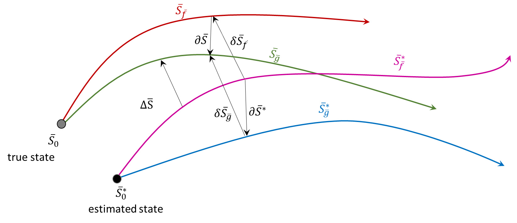
The following figure shows the evolution of two states, an estimated initial state  $$\bar S^*_0$$ and a true initial state  $$\bar S_0$$, each under the action of two right-hand sides  $$\bar f$$ (estimated model) and  $$\bar g$$ (true model).  In this figure, $$\delta \bar S$$ is the state variation, $$\partial \bar S$$ is the model variation, $$\Delta \bar S$$ is the total variation.

The key assumption is that both the state and model variations lead to small deviations in the evolution.  If this assumption holds, a linearized equation of motion for the state and total variations can be derived.  Since the true state and model are not none for physical systems (as opposed to mathematical models) it is most useful to ultimately express all the deviations in terms of the state deviation under the estimated model, since this is the one most easily probed.  The linearization is relatively easy and will be done for state and model variations first and then will be combined for the total variation.

State Variation

Start with the basic relation $$\delta \bar S = \bar S – \bar S^*$$.  To calculate the differential equation for the state variation apply the time derivative to both sides

\[ \frac{d}{dt} \delta \bar S = \frac{d}{dt} \left[ \bar S – \bar S^* \right] \]

and use the original equation of motion to eliminate the derivatives of the state in favor of the right-hand sides of the differential equation.

\[ \frac{d}{dt} \delta \bar S = \bar f(\bar S) – \bar f (\bar S^*) \]

Since the model is the same in both cases, it really doesn’t matter which model is used but using $$\bar f$$ will be convenient later.  Finally, express the true state in terms of the estimate state and the state deviation

\[ \frac{d}{dt} \delta \bar S = \bar f(\bar S^* + \delta \bar S) – \bar f(\bar S^*) \]

and expand

\[ \frac{d}{dt} \delta \bar S = \left. \frac{\partial \bar f}{\partial \bar S} \right|_{\bar S^*} \delta \bar S \; .\]

Note that the matrix $$A \equiv \left. \frac{\partial \bar f}{\partial \bar S} \right|_{\bar S^*}$$ is evaluated along the estimated trajectory (although in this case either will suffice) and is, in general, time-varying because of it.

Model Variation

The equation of motion for the model variation is the most analytically intractable of the variations and does not lead directly to a linear equation.  To evaluate it, take the time derivative of the definition of the model variation

\[ \frac{d}{dt} \partial \bar S = \frac{d}{dt} \left[ \bar S_{\bar g} – \bar S_{\bar f} \right] \; . \]

Replace the derivatives on the right gives

\[ \frac{d}{dt} \partial \bar S = \bar g (\bar S) – \bar f(\bar S) \equiv \bar \eta_0(\bar S) \; .\]

This is as far as one can go with the general structure.  But it is usually argued that if the actual forces are not producing a discernable signal (for if they were, they could be inferred from the motion) then $$\bar \eta_0$$ can be thought of as an inhomogeneous noise term.  We will make such an argument and assume this property.

Total Variation

From the figure there are two equally valid definitions of the total variation in terms of true state

\[ \Delta \bar S = \delta \bar S_{\bar f} + \partial \bar S \]

and in terms of the estimated state

\[ \Delta \bar S = \delta \bar S_{\bar g} + \partial \bar S^* \; . \]

Equating, rearranging, and taking the time derivative yields

\[ \frac{d}{dt} \delta \bar S_{\bar g} = A \delta \bar S_{\bar f} – \bar \eta^*_0 – \bar \eta_0 \; \]

One last approximation is needed.  Much like the argument above, it is based on a plausibility and not on a rigorous linearization.  This argument says that if the differences between the two force models are small enough to regard the model variations to be noise-like, then for all practical considerations the state variations are approximately the same.

Thus the final equation is

\[ \frac{d}{dt} \delta \bar S_{\bar f} = A \delta \bar S_{\bar f} + \bar \eta \; \]

where $$\bar \eta$$ is a collected noise term (with an appropriate and insignificant sign change).  It should be emphasized that this final equation is not rigorous correct but has been used by control engineers successful and so is worth studying.

In this post, the focus shifts from looking at the basic properties of the Laplace Transform to the application of it to dynamical systems of the form

\[ \frac{d}{dt} \bar S = A \bar S \; ,\]

where the matrix $$A$$ can be time-varying but does not depend on the state $$\bar S$$.

To be sure, some differential equations were already touched upon in passing in earlier posts, but this was done more as a way to motivate the possible transforms that would result and which would require a subsequent inverse rather than being examined in their own right.

As a prototype for multi-variable dynamical systems and a prelude to the general theory, this column will look at the application of the Laplace Transform in the simplest multi-variable structure – the simple harmonic oscillator (SHO). This tried and true system should always be the first one explored based on one simple fact – if the theory is not understandable or workable for this fundamental system then it won’t be understandable or workable for any other application.

The familiar state for the SHO is given by:

\[ \bar S = \left[ \begin{array}{c} x(t) \\ v(t) \end{array} \right] \; \]

and its corresponding equation of motion

\[ \frac{d}{dt} \left[ \begin{array}{c} x \\ v \end{array} \right] = \left[ \begin{array}{cc} 0 & 1 \\ -\omega_0^2 & 0 \end{array} \right] \left[ \begin{array}{c} x \\ v \end{array} \right] \; ,\]

where the matrix $$A$$ is given by

\[ A = \left[ \begin{array}{cc} 0 & 1 \\ -\omega_0^2 & 0 \end{array} \right] \; .\]

Taking the Laplace Transform of the oscillator’s equation of motion (using the properties established in earlier posts) yields

\[ \left[ \begin{array}{c} s X(s) – x_0 \\ s V(s) – v_0 \end{array} \right] = \left[ \begin{array}{cc} 0 & 1 \\ -\omega_0^2 & 0 \end{array} \right] \left[ \begin{array}{c} X(s) \\ V(s) \end{array} \right] \; .\]

Note that, as expected, the differential equation now becomes a (linear) algebraic equation.

Some basic re-arrangement leads to the following matrix equation

\[ (s Id – A) \left[ \begin{array}{c} X(s) \\ V(s) \end{array} \right] = \left[ \begin{array}{c} x_0 \\ v_0 \end{array} \right] \; ,\]

where $$Id$$ is the $$2×2$$ identity matrix.

The solution to this equation is obtained by finding the inverse of the matrix $$s Id – A$$.

\[ \left[ \begin{array}{c} X(s) \\ V(s) \end{array} \right] = (s Id – A)^{-1} \left[ \begin{array}{c} x_0 \\ v_0 \end{array} \right] \; .\]

It is convenient to define

\[ M = s Id – A = \left[ \begin{array}{cc} s & -1 \\ \omega_0^2 & s \end{array} \right] \; .\]

The inverse then follows from the usual formula for a $$2×2$$ matrix

\[ M^{-1} = \frac{1}{s^2 + \omega_0^2} \left[ \begin{array}{cc} s & 1 \\ -\omega_0^2 & s \end{array} \right] \; ,\]

where the pre-factor is $$1/det(M)$$.

Multiply the right-hand side out leads to the following expressions for $$X(s)$$

\[ X(s) = \frac{s x_0}{s^2 + \omega_0^2} + \frac{v_0}{s^2 + \omega_0^2} \; \]

and $$V(s)$$

\[ V(s) = -\frac{x_0 \omega_0^2 }{s^2 + \omega_0^2} + \frac{s v_0}{s^2 + \omega_0^2} \; .\]

The last piece is to take the inverse Laplace Transform of the individual components to get

\[ x(t) = x_0 \cos(\omega_0 t) + \frac{v_0}{\omega_0} \sin(\omega t) \; \]

and

\[ v(t) = -x_0 \omega_0 \sin(\omega_0 t) + v_0 \cos(\omega t) \; ,\]

which, happily, are the expected results.

Next week, I’ll begin my examination of the general theory use in controls engineering.

One of the most peculiar things about the Laplace Transform, specifically, and the integral transforms, in general, is the very nonintuitive behavior that results when performing either the forward or inverse transform on the product of two functions. Up to this point, only very special cases have been covered – cases where the results of the product could be determined easily from the definition of the transform itself (e.g. $${\mathcal L}[t f(t)]$$) or cases where the product of two transforms $$G(s)F(s)$$ resulted in a trivial inverse due to some property of the Laplace Transform that allowed for clever manipulation.

Unfortunately, cleverness has a limit. So this week’s column will be looking at the general theory of the transform/inverse-transform of the product of two functions. This leads directly to the convolution integrals.

The first thing to look at is the case where the product of a set of Laplace Transforms fail to inspire cleverness on our part. This situation can easily arise when solving a differential equation such as

\[ x”(t) + \omega^2 x(t) = f(t), \; \; x(0) = 0, \; x'(0) = 0 \; ,\]

which is the driven simple harmonic oscillator with homogenous initial conditions.

Application of the Laplace transform leads to

\[ X(s) = \frac{F(s)}{s^2 + \omega^2} \]

as the solution that we wish to find by the inverse Laplace Transform, where $$F(s) = {\mathcal L}[f(t)]$$.

For certain forms of $$F(s)$$ (usually simple ones) the inverse Laplace Transform can be done using the properties already established. But clearly, an arbitrary form requires a little something more.

The little bit more comes in the form of the convolution $$f*g$$, defined as

\[ (f*g)(t) = \int_{0}^{t} d\tau \, f(t-\tau) g(\tau) \; .\]

The convolution has exactly the same form as the kernel integration that arises in the study of the Green’s function and has been dealt with in detail in other entries of this blog.

The reason the convolution is useful can be seen if we examine its Laplace Transform

\[ {\mathcal L}[(f*g)(t)] = \int_0^{\infty} dt \, (f*g)(t) e^{-st} = \int_0^{\infty} dt \, \int_0^t d\tau \, f(t-\tau) g(\tau) e^{-st} \; .\]

The inner integral can have the same limits of integration as the outer one if we introduce the Heaviside step function

\[ H(x) = \left\{ \begin{array}{l} 0 \; \; x<0 \\ 1 \; \; x \geq 0 \end{array} \right. \; \] to get \[ {\mathcal L}[(f*g)(t)] = \int_0^{\infty} dt \int_0^{\infty} d\tau \, f(t-\tau) g(\tau) H(t-\tau) e^{-st} \; . \] Next switch the order of integration \[ {\mathcal L}[(f*g)(t)] = \int_0^{\infty} d\tau \, g(\tau) \int_0^{\infty} dt f(t-\tau) H(t-\tau) e^{-st} \; \] and then substitute $$\lambda = t – \tau$$ in the inner integral (realizing that $$\tau$$ is regarded as a parameter) to get \[ {\mathcal L}[(f*g)(t)] = \int_0^{\infty} d\tau \, g(\tau) \int_0^{\infty} d\lambda f(\lambda) H(\lambda) e^{-s(\lambda+\tau)} \; .\] Separate the exponential into two pieces; the first solely involving $$\tau$$ and the second solely involving $$\lambda$$ and bring the last factor out of the inner integral to get \[ {\mathcal L}[(f*g)(t)] = \int_0^{\infty} d\tau \, g(\tau) e^{-s\tau} \int_0^{\infty} d\lambda f(\lambda) H(\lambda) e^{-s\lambda} \; .\] The final two steps are, first, to realize that the $$H(\lambda)$$ term in the inner integral is always $$1$$ and therefore can be dropped and, second, to recognize that each integral is a Laplace Transform. Finally, we arrive at \[ {\mathcal L}[(f*g)(t)] = G(s) F(s) \; .\] At first glance, it may seem that there is a problem with the above relation. Clearly the order of the products on the right-hand side doesn’t matter $$G(s)F(s) = F(s)G(s)$$. In contrast, the left-hand side doesn’t appear to support commutivity of $$f$$ and $$g$$. However, appearances are deceiving, and it is a short proof to show that all is well. Start with the first form of the equation \[ (f*g)(t) = \int_{0}^{t} d \tau \, f(t-\tau) g(\tau) \] and make the substitution $$t-\tau = u$$ (which implies $$d\tau = -du$$) to transform the right-hand side to \[ (f*g)(t) = \int_{t}^{0} (-du) \, f(u) g(t-u) = \int_{0}^{t} du \, g(t-u) f(u) = (g*f)(t) \; .\] Returning to the original differential equation we started to solve, we find that \[ x(t) = \int_0^t \frac{sin(\omega(t-\tau))}{\omega} f(t) \; , \] which is exactly the expected result based on the Green’s function method. Some other interesting properties of the convolution operator is that it is distributive \[ f*(g+h) = f*g + f*h \] and that it is associative \[ (f*g)*h = f*(g*h) \; .\]

Both of these are easy to prove as well. For the first relation

\[ f*(g+h) = \int_0^t d\tau \, f(t-\tau) \left[ g(\tau) + h(\tau) \right] \\ = \int_0^t d\tau \, f(t-\tau) g(\tau) + \int_0^t \, f(t-\tau) h(\tau) = f*g + f*h \; .\]

For the second relation, things are a bit harder. And we’ll take it on faith for now. Having disposed of the forward transform theory in fine order, it is natural to ask about the inverse transform. Here the work is much simpler. There is an analogous expression that states \[ f(t) g(t) = {\mathcal L}^{-1}[ F(s) * G(s) ] \] which not particularly useful but follows just from the simple changing of the identity of the symbols in the analysis above. Finally, one might ask about the Laplace Transform of the product of two arbitrary (but transformable) functions $$f(t) g(t)$$. Here the theory is not so attractive. The transform is given abstractly as

\[ {\mathcal L}[f(t) g(t)] = \frac{1}{2 \pi i} \int_{c-i\infty}^{c+i\infty} \, dp G(s-p) F(p) \\ = \frac{1}{2 \pi i} \int_{c-i\infty}^{c+i\infty} \, dp F(s-p) G(p) \; ,\]

where the real constant $$c$$ is the largest of the abcissa of convergence of $$f(t)$$ and $$g(t)$$. This form is really dreadful and it demonstrates that there is no free lunch anywhere. The transform approach may make certain computations easier but other things are more complex. There are always trade-offs. To see how this comes miserable state-of-affairs about start with the basic definition of the Laplace Transform of the product \[ {\mathcal L}[f(t) g(t)] = \int_0^\infty dt \, f(t) g(t) e^{-st} \; .\] Now assume that both $$f(t)$$ and $$g(t)$$ individually have Laplace transforms so that the inverses \[ f(t) = \frac{1}{2 \pi i} \int_{c_f – i \infty}^{c_f + i \infty} ds \, F(s) e^{st}, \;\; \mbox{for} \; t > 0 \]

and

\[ g(t) = \frac{1}{2 \pi i} \int_{c_g – i \infty}^{c_g + i \infty} ds \, G(s) e^{st}, \;\; \mbox{for} \; t > 0 \]

exist and that $$c_f$$ and $$c_g$$ are the abcissa of convergence associated with the functional form of $$f(t)$$ and $$g(t)$$, respectively.

First substitute the inverse expression for $$f(t)$$ into the basic definition to get

\[ {\mathcal L}[f(t) g(t)] = \int_0^\infty dt \, \left\{ \frac{1}{2 \pi i} \int_{c_f – i \infty}^{c_f + i \infty} dp \, F(p) e^{pt} \right\} g(t) e^{-st} \; .\]

Since the integrals are assumed to be convergent, trading the order of integration is allowed, giving

\[ {\mathcal L}[f(t) g(t)] = \frac{1}{2 \pi i} \int_{c_f – i \infty}^{c_f + i \infty} dp \, F(p) \int_0^\infty dt \, e^{-(s-p)t} g(t) \; .\]

The inner integral can be simplified to

\[ \int_0^\infty dt \, e^{-(s-p)t} g(t) = G(s-p) \; \]

and so we arrive at

\[ {\mathcal L}[f(t) g(t)] = \frac{1}{2 \pi i} \int_{c_f – i \infty}^{c_f + i \infty} dp \, F(p) G(s-p) \; .\]

In a similar fashion (switching the order in which $$f(t)$$ and $$g(t)$$ are handled), we also get the analogous expression with the roles of $$F$$ and $$G$$ reversed.

Next week, I’ll be looking at solving systems of equations using the Laplace Transform, which will be a prelude to a brief dip into modern control theory.

There are two theorems that are of particular interest not so much for their general applicability but for their use as safety checks on the solutions obtained with the Laplace Transform: the Initial Value Theorem and the Final Value Theorem. Both of these theorems produce a particular value (either initial or final) of the underlying signal $$f(t)$$ from a limiting process on the signal’s Laplace Transform $$F(s)$$.

A moment’s reflection helps to understand why such interrogations are useful.

With respect to the Initial Value Theorem, the argument goes as follows. When searching for the solution of a differential equation using the Laplace Transform, derivatives of the unknown and sought-for signal $$f(t)$$ are replaced by algebraic quantities proportional to some power of the frequency variable $$s$$ times $$F(s)$$ or some power of $$s$$ multiplying the initial conditions $$f(0)$$, $$f'(0)$$. and so on. Once the explicit values of the initial conditions are substituted into the transformed equation, many algebraic manipulations follow, each one typically elementary but each on fraught with the possibility of mistake. When the final form of $$F(s)$$ is obtained, it is comforting to be able to tease back out that the original initial conditions are still in there; unmolested by the many steps used to obtain the final form.

With respect to the Final Value Theorem, the argument takes on a different caste entirely. Generally, even though we don’t know the explicit form of the signal $$f(t)$$ (otherwise it wouldn’t be unknown) we usually have a general notion of what to expect. The final solution may be oscillatory or it may damp out or it may tend to a limiting value and so on. The Final Value Theorem provides a simple way to see what the signal $$f(t)$$ is doing a long time into the future without the bother of having to perform an inverse Laplace Transform.

Thus the Initial Value Theorem provides a way of looking at the very start of the transient behavior of the signal $$f(t)$$ while the Final Value Theorem provides a way of determining some of its steady state characteristics. Both theorems are relatively easy to prove.

To prove the Initial Value Theorem, start with the property of the Laplace Transform

\[ {\mathcal L}\left[ \frac{d}{dt} f(t) \right] = s F(s) – f(0) \; .\]

Now examine the limit of the left-hand side as $$s \rightarrow \infty$$.

\[ \lim_{s \rightarrow \infty} {\mathcal L}\left[ \frac{d}{dt} f(t) \right] = \lim_{s \rightarrow \infty} \int_{0}^{\infty} dt \, \frac{d f(t)}{dt} e^{-st} \; . \]

Agreeing that the lower limit of the integral is approach from above (i.e. $$0^+$$), the limit with respect to $$s$$ can be brought inside the integral giving

\[ \int_{0}^{\infty} dt \, \frac{d f(t)}{dt} \lim_{s \rightarrow \infty} e^{-st} = \int_{0}^{\infty} dt \, \frac{d f(t)}{dt} \cdot 0 = 0 \; .\]

So the Initial Value Theorem is

\[ f(0) = \lim_{s \rightarrow \infty} s F(s) \; .\]

In a completely similar fashion, the initial value for the time derivative $$\dot f(0)$$ is obtained from the Laplace Transform identity

\[ {\mathcal L}\left[ \frac{d^2}{dt^2} f(t) \right] = s^2 F(s) – s f(0) – \dot f(0) \]

giving

\[ \dot f(0) = \lim_{s \rightarrow \infty} \left( s^2 F(s) – s f(0) \right) \]

once the appropriate limit on $$s$$ is taken.

To prove the Final Value Theorem, start with the same Laplace Transform property used for the Initial Value Theorem but take the limit as $$s \rightarrow 0$$:

\[ \lim_{s \rightarrow 0} \int_{0}^{\infty}dt \, \frac{d f(t)}{dt} e^{-st} = \lim_{s \rightarrow 0} s F(s) – f(0) \; . \]

Next take the limit inside the integral to transform the left-hand side as

\[ \int_{0}^{\infty}dt \, \frac{d f(t)}{dt} \lim_{s \rightarrow 0} e^{-st} = \int_{0}^{\infty}dt \, \frac{d f(t)}{dt} \cdot 1 \\ = \left. f(a) \right|_{a \rightarrow \infty} – f(0) \equiv f(\infty) – f(0) \; .\]

Combining yields

\[ f(\infty) – f(0) = \lim_{s \rightarrow 0} \left( s F(s) – f(0) \right) \]

or

\[ f(\infty) = \lim_{s \rightarrow 0} s F(s) \; .\]

Having proved both of these theorems, it will prove useful to look at an example.

Suppose we have the following differential equation

\[ \ddot x (t) + 5 x(t) = e^{-7t} \; \; , x(0) = 11 \;\; , \dot x(0) = 13 \; .\]

The corresponding Laplace Transform is given by

\[ F(s) = {{11\,s^2+13\,\left(s+7\right)+77\,s+1}\over{s^3+7\,s^2+5\,s+35}} \; \]

Finding the inverse Laplace Transform is not particularly inviting due to the complex nature of the denominator and we don’t want to spend time trying to do this if we’ve made an algebraic error. Also, from the structure of the original equation, we expect that the final signal should be a combination of oscillatory motion (due to the motion under the homogenous equation $$\ddot x + 5 x = 0$$) plus some motion that tends to follow the driving force, which damps to zero in the limit of large $$t$$.

So the first step is to see if the initial conditions are still contained in the Laplace Transform.

The Initial Value Theorem says that

\[ \lim_{t \rightarrow 0} f(t) = \lim_{s \rightarrow \infty} s F(s) \; .\]

Applying this to the particular form above gives

\[ \lim_{s \rightarrow \infty} s F(s) = \lim_{s \rightarrow \infty} {{11\,s^3+13 s\,\left(s+7\right)+77\,s^2+s}\over{s^3+7\,s^2+5\,s+35}} = 11 \; . \]

So far so good!

Now let’s look for the initial conditions on $$\dot x$$.

\[ \lim_{t \rightarrow 0} \dot f(t) = \lim_{s \rightarrow \infty} \left( s^2 F(s) – s f(0) \right) = 13 \; ,\]

which is most easily seen by noticing that the only term that can survive is the leading term $$11 s^4$$ which becomes in the limit $$11 s$$ which is exactly equal to the term subtracted off due to the Initial Value Theorem.

Finally, let’s look at the long-time or steady-state behavior (assuming that it exists). The Final Value Theorem when applied in this case yields

\[ \lim_{s \rightarrow 0} s F(s) = \lim_{s \rightarrow 0} {{11\,s^3+13 s\,\left(s+7\right)+77\,s^2+s}\over{s^3+7\,s^2+5\,s+35}} = 0 \; .\]

This answer is reasonable as the forcing function will have a tendency to damp out all motion as $$t$$ gets large.

As a check, the inverse Laplace Transformation (courtesy of wxMaxima) yields

\[x(t) = {{709\,\sin \left(\sqrt{5}\,t\right)}\over{54\,\sqrt{5}}}+{{593\,\cos \left(\sqrt{5}\,t\right)}\over{54}} + {{e^{-7\,t}}\over{54}}\]

which clearly has a limit of $$0$$ as $$t$$ gets large.

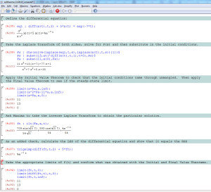
For reference, the wxMaxima steps for this analysis are:

Next week, I’ll be looking at convolution integrals and the products of transforms.

Having established some attractive properties of the Laplace Transform that make solving linear differential equations relatively easy, the next logical question to ask is, under what conditions does the Laplace transform actually exist? In answering this, I will follow closely the individual arguments found in Modern Control Engineering by Katsuhiko Ogata, but I’ll be modifying their context to aim at the larger question of the relation between the Laplace and Fourier Transforms.

The first step into understanding what functions are Laplace transformable is to look at the basic definition

\[ {\mathcal L}[f(t)] = \int_0^{\infty} dt \, e^{-st} f(t) \; .\]

The Laplace Transform will only exist when the integral on the right-hand side is convergent. Note that the integral restricts itself to the portion of $$f(t)$$ that falls in the range $$[0,\infty]$$. Since the Laplace Transform doesn’t ask or care about the behavior of $$f(t)$$ for values of $$t < 0$$, the common prescription is to define $$f(t) = 0$$ for $$t < 0$$.

It is a fair question to ask why this requirement is imposed if the the Laplace Transform doesn’t ‘see’ the values of $$f(t)$$ for $$t<0$$. Later on in this column, a relationship between the Fourier and Laplace Transforms presents a plausible justification. For now, let's just say that there are matters of causality that say a signal didn't exist in perpetuity and, thus, at some point in the past it had to turn on. That is what is meant by $$t=0$$.

Of course, there are deep philosophical problems with this point of view, but they don’t touch on the day-to-day workings of the physicist or controls engineer.

So, the operative question is, what type of function, so restricted, has a convergent integral? The class of functions that allow the integral to exist are said to be of exponential order. Operationally, this means that

\[ \lim_{t\rightarrow0} \, e^{-\gamma} |f(t)| = 0 \]

for some positive real number $$\gamma$$ ($$s = \gamma + i \omega$$). If the limit is such that it tends to $$0$$ for $$\gamma > \sigma_c$$ and tends to $$\infty$$ for $$\gamma < \sigma_c$$, the real, positive number $$\sigma_c$$ takes on the name the abscissa of convergence. What this is telling us is that the Laplace Transform only converges when the real part of $$\Re(s) = \gamma$$ is greater than $$\sigma_c$$.

As we will discuss in the example below, this means that $$\gamma$$ must be greater than the right-most pole of the transform $$F(s) = \int_0^{\infty} dt \, e^{-st} f(t)$$.

Some additional words are in order. Functions that increase faster than an exponential do not have Laplace Transforms. The most-oft cited counter-example is the function $$e^{t^2} \; \forall t > 0$$. Note that $$e^{t^2}$$ is a perfectly fine signal if it is defined with compact support, such that it is zero for times $$t>t_{max}$$.

There is an obvious concern that arises at this point. Since the purpose of the Laplace Transform is to turn differential equations into algebraic equations, there is no easy way to restrict the resulting solution to that algebraic equation to have one simple pole. For example, the differential equation $$\ddot x(t) + 3 \dot x(t) + 2 x(t) = f(t)$$ has a Laplace-Transformed left-hand-side of $$s^2 + 3s + 2 = (s+2)(s+1)$$ times $${\mathcal L}[x(t)] \equiv X(s)$$. Assuming the Laplace Transform of $$x(t)$$ and $$f(t)$$ exists, then the following algebraic equation corresponds to the original differential equation with homogeneous initial conditions:

\[ (s+2)(s+1)X(s) = F(s)\; . \]

Solving this for $$X(s)$$ sets before us the task of finding an inverse Laplace Transform for

\[ X(s) = \frac{F(s)}{(s+2)(s+1)} \; .\]

Even assuming that $$F(s)$$ has no poles of its own, the above analysis would suggest that the minimum value of $$\Re(s)$$ would be $$\Re(s)=-1+\epsilon$$, where $$\epsilon$$ is a small positive number. This condition restricts $$s$$ to a portion of the complex plane that doesn’t include the other pole. But the $$s$$ value at the other pole corresponds to physically allowed frequencies, so, how does one reconcile this?

To answer this question, I quote a passage from Ogata’s book:

So, since the theory is now well supported, let’s return to the question as to whether or not the restriction of $$f(t) = 0 \; \forall t < 0$$ is needed. To try to justify this, bring in the Fourier Transform (this argument is based on the ideas of P.C. Chau).

The basic form of the Fourier Transform is

\[ {\mathcal F}[f(t)] = \int_{-\infty}^{\infty} dt \, f(t) e^{-i \omega t} \equiv F(\omega) \]

with the inverse transform being

\[ f(t) = \frac{1}{2\pi} \int_{-\infty}^{\infty} d\omega \, F(\omega) e^{i\omega t} \; .\]

Now consider the Fourier Transform of the special form of

\[ f(t) = e^{-\gamma t} g(t) \; .\]

The identity $$f(t) = {\mathcal F}^{-1}\left[{\mathcal F}[f(t)] \right]$$ becomes

\[ f(t) \frac{1}{2\pi} \int_{-\infty}^{\infty} d \omega \, \left[ \int_{-\infty}^{\infty} d \tau \, f(\tau) e^{-i \omega \tau} \right] e^{i\omega t} \]

and

\[ e^{-\gamma t} g(t) = \frac{1}{2\pi} \int_{\infty}^{\infty} d \omega \, \int_{-\infty}^{\infty} d \tau \, e^{-\gamma \tau} g(\tau) e^{-i \omega \tau} e^{i \omega t} \; .\]

Bringing the $$e^{-\gamma t}$$ over to the right-hand side and rearranging gives

\[ g(t) = \frac{1}{2\pi} \int_{\infty}^{\infty} d \omega \, e^{(i\omega + \gamma)t} \int_{-\infty}^{\infty} d \tau \, e^{-(i\omega + \gamma) \tau} g(\tau) .\]

Now define the Laplace variable $$s = \gamma + i \omega$$ from which $$d\omega = ds/i$$ and substitute back in to change the outer integral to get the final form

\[ g(t) = \frac{1}{2\pi} \int_{\gamma – i\infty}^{\gamma + i \infty} d s \, e^{s t} \int_{-\infty}^{\infty} d \tau \, e^{-s \tau} g(\tau) .\]

The inner integral will not converge unless $$\tau$$ is restricted so that it is always positive. So, here is a plausible, well-supported argument for always defining $$f(t)$$ in a piece-wise fashion so that it is zero in the range $$t<0$$.

A couple of final notes. The contour implied in the final integral is known as the Bromwich contour. It is rarely used in practice to compute an inverse Laplace Transform with the usual technique being a combination of a clever use of already tabulated transforms and the use of partial fraction decomposition. Another technique for obtaining the inverse Laplace Transform also exists that does not depend on either of these approaches and I’ll devote some future space to examining it.

Next week, I’ll be taking a look at some additional properties of the Laplace Transform that make convenient the separation of transient and steady-state effects.

As regular readers know, time evolution of classical and quantum systems is a popular topic on this blog, forming a major thread of the columns to date. But the majority of column space dealing with the initial value problem has either been devoted to time domain analysis or, less frequently, with frequency domain techniques that fall under the Fourier Transform heading. This week starts what will be a lazy meandering through the Laplace Transform.

The Laplace Transform is a favorite of engineers, specifically ones who have to work with feedback control, and it would be worth exploring simply for that reason alone. However, it is also curious that its existence is almost wholely absent from the standard training for physicists. Exactly why the latter tend to use the Fourier transform at the expense of all else can be confidently guessed at (the Fourier Transform seems to be built into Quantum Mechanics) but a deeper understanding will result simply by comparing and contrasting the two methods.

Well before that last goal can be reached, the Laplace Transform must be examined on its own merits.

The Laplace Transform is a functional that maps input functions to output functions via

\[ {\mathcal L}[f(t)] = \int_0^{\infty} dt \, e^{-st} f(t) \; .\]

It is often written in a shorthand way as

\[ {\mathcal L}[f(t)] \equiv F(s) \; , \]

since this notation makes for convenient manipulation.

The properties of the Laplace Transform that make it so useful can be summarized as:

1. it is a linear transformation,
2. it turns operations of differentiation and integration into algebraic operations,
3. incorporates the initial conditions seamlessly, and
4. is general, thus affording a single approach applicable to an extraordinary wide range of situations.

One caveat is needed on point 4. All Laplace Transforms can only be applied when the system obeys a set of linear evolution equations. In this regard, it is unable to tackle the range and scope of problems that the Lie Series can deal with but its convenience for linear (or linearized) systems makes it a favorite of the controls engineer.

Let’s look at the first 3 points in more detail. For an operation $${\mathcal O}$$ to be linear, the following relationship must hold

\[ {\mathcal O}[a F + b G] = a {\mathcal O}[F] + b {\mathcal O}[G] \; ,\]

where $$a,b$$ are constants and $$F,G$$ are functions. The properties of the integral insure that the Laplace Transform is linear as follows

\[ {\mathcal L}[a f(t) + b g(t) ] = \int_0^{\infty} dt \, e^{-st} \left( a f(t) + b g(t) \right) \\ = a \int_0^{\infty} dt \, e^{-st} f(t) + b \int_0^{\infty} dt \, e^{-st} g(t) \\ = a {\mathcal L}[f(t)] + b {\mathcal L}[g(t)] \; .\]

The Laplace Transform is a machine which takes an input function and maps it to an output function. Differentiation is also a machine that maps input functions to output functions. It’s logical to ask how do these two operations interact.

To figure this out, feed the derivative of a function $$f'(t)$$ into the Laplace Transform.

\[ {\mathcal L}[f'(t)] = \int_0^{\infty} dt \, e^{-st} f'(t) \]

and integrate by parts to move the derivative off of $$f(t)$$ and onto the exponential. This gives

\[ {\mathcal L}[f'(t)] = \left. e^{-st} f(t) \right|_0^{\infty} – \int_0^{\infty} dt \, \left( \frac{d}{dt} e^{-st} \right) f(t) \; , \]

which simplifies to

\[ {\mathcal L}[f'(t)] = -f(0) + \int_0^{\infty} dt \, s e^{-st} f(t) = s F(s) – f(0) \; .\]

The same steps can be followed for higher order derivatives but a more useful way is to simply use an induction argument. Define a second derivative to be the derivative of first derivative and apply the theorem twice.

\[{\mathcal L}[f^{\prime\prime}(t)] = {\mathcal L}[(f'(t))’] = s {\mathcal L}[f'(t)] – f'(0) = s^2 F(s) – s f(0) – f'(0) \; \]

This process can be repeated as often as desired yielding the general form

\[ {\mathcal L}\left[ \frac{d^n}{dt^n} f(t) \right] = s^n F(s) – s^{n-1} f(0) – s^{n-2} f^{(1)}(0) – s^{(n-3)} f^{(2)}(0) – \ldots \; ,\]

where

\[ f^{(n)}(0) = \left. \frac{d^n}{dt^n} f(t) \right|_0 \; .\]

Likewise, the Laplace Transform takes integrals of functions to algebraic relations as well. As in the derivative case, start with the most basic form of

\[{\mathcal L}\left[ \int dt’ \, f(t’) \right] = \int_0^{\infty} dt \; e^{-st} \int dt’ \, f(t’) \; . \]

An application of an integration-by-parts is next employed with

\[ dV = e^{-st} \implies V = – \frac{1}{s} e^{-st} \]

and

\[ U = \int dt’ \, f(t’) \implies \frac{dU}{dt} f(t) \; , \]

yielding

\[ \int_0^{\infty} dt \, e^{-st} \int dt’ \, f(t’) = \left.-\frac{1}{s} e^{-st} \int dt’ \, f(t’) \right|_0^{\infty} – \int_0^{\infty} \left(-\frac{1}{s} \right) e^{-st} f(t) \; \]

This expression simplifies to

\[ {\mathcal L}\left[ \int dt’ \, f(t’) \right] = \frac{f^{(-1)}(0)}{s} + \frac{1}{s} F(s) \; ,\]

where $$f^{(-1)}(0) = \int dt’ \, f(t’) \left.\right|_0$$ is a convenient short-hand.

Repeated applications yields the generalization

\[ {\mathcal L}\left[ \int dt’ \, \int dt^{\prime\prime} \, \ldots \int dt^{(n)} \, f(t^{(n)})\right] = \frac{f^{(-n)}(0)}{(s)} + \frac{f^{(-n+1)}(0)}{(s^2)} \\ + \ldots + \frac{F(s)}{s^n} \; .\]

In contrast, the Laplace Transform of products and divisions, results in derivatives and integrations in the $$s$$-space.

First consider multiplication of $$f(t)$$ by some power of $$t$$:

\[ {\mathcal L}[t f(t)] = \int_0^{\infty} dt \, e^{-st} t f(t) \; .\]

Recognize that

\[ \frac{d}{dt} \left( e^{-st} \right) = -t e^{-st} \;.\]

Thus

\[ {\mathcal L}[t f(t)] = -\int_0^{\infty} dt \, \frac{d}{ds} \left( e^{-st} \right) f(t) = -\frac{d}{ds} \int_0^{\infty} dt \, e^{-st} f(t) = -\frac{d}{ds} F(s) \; .\]

This is easily generalized to any arbitrary power to yield

\[ {\mathcal L}[t^n f(t) ] = (-1)^n \frac{d^n}{ds^n} {\mathcal L}[f(t)] = (-1)^n \frac{d^n}{ds^n} F(s) \; .\]

As the last piece, let’s look at division by a power of $$t$$, starting with the simplest case

\[ {\mathcal L}[f(t)/t] = \int_0^{\infty} dt \, e^{-st} f(t)/t \; .\]

Recognizing that

\[ \int_s^{\infty} ds’ \, e^{-s’ t} = e^{-st}/t \]

allows for the Laplace Transform to become

\[{\mathcal L}[f(t)/t] = \int_0^{\infty} dt \int_s^{\infty} ds’ \, e^{-s’ t} = \int_s^{\infty} ds’ \, F(s’) \; .\]

This is also easily generalized to arbitrary powers to yield

\[{\mathcal L}[f(t)/t^n] = \int_s^{\infty} ds’ \, \int_{s’}^{\infty} ds^{\prime\prime} \ldots \int_{s^{(n-1)}}^{\infty} ds^{(n)} F(s(n)) \;.\]

Next week, I’ll take a look at what functions possess a Laplace Transform and how the Laplace Transform relates to the Fourier Transform.

One of the topics touched on in some of the recent posts about Lie series was the idea that a non-autonomous equation can be handled relatively easily in the Lie series framework by enlarging the state space from $$2N$$-dimensions to $$2N+1$$-dimensions. I thought it would be beneficial to see how this is done in an explicit example where the actual equations of motion can be solved analytically.

The candidate for this is treatment is an otherwise free particle, moving in one dimension, subjected to a time varying force. The reason is for this is that the second-order Newtonian, first-order state space, and Green’s functions methods (both time and frequency space) all provide the same answer with relatively little work.

The Newton Method

The Newtonian equation of motion is

\[ \frac{d^2}{dt^2} x = F(t) \; .\]

To get a solution, integrate twice with respect to time to arrive at

\[ x(t) = x_0 + v_0 (t – t_0) + \int_{t_0}^{t} dt’ \int_{t_0}^{t’} dt” F(t”) \; , \]

where $$x_0$$ and $$v_0$$ are the initial position and velocity at time $$t_0$$.

This solution isn’t particularly useful and a much better form results after an integration-by-parts. The usual form of integration-by-parts $$ \int dU \, V = U V – \int U dV $$ is carried out by identifying:

\[ dU = dt’ \]

and

\[ V(t’) = \int_{t_0}^{t’} dt” F(t”) \; \]

Plugging these in yields

\[ x(t) = x_0 + v_0 (t – t_0) + (t-t_0) \int_{t_0}^{t} dt” F(t”) – \int_{t_0}^{t} dt’ (t’-t_0) F(t’) \; \]

or, upon combining the last two terms

\[ x(t) = x_0 + v_0 (t – t_0) + \int_{t_0}^{t’} dt’ (t-t’) F(t’) \; .\]

State Space Method

An alternative way to arrive at the same solution is in the state-space picture. Here the equation of motion is given by

\[ \frac{d}{dt} \left[ \begin{array}{c} x \\ v \end{array} \right] = \left[ \begin{array}{c} x \\ v \end{array} \right] = \left[ \begin{array}{cc} 0 & 1 \\ 0 & 0 \end{array} \right] \left[ \begin{array}{c} x \\ v \end{array} \right] + \left[ \begin{array}{c} 0 \\ F(t) \end{array} \right] . \]

The form of the process matrix makes the construction of the state transition matrix particularly easy. To wit

\[ A = \left[ \begin{array}{cc} 0 & 1 \\ 0 & 0 \end{array} \right] \; ,\]

\[ A^2 = \left[ \begin{array}{cc} 0 & 1 \\ 0 & 0 \end{array} \right] \left[ \begin{array}{cc} 0 & 1 \\ 0 & 0 \end{array} \right] = \left[ \begin{array}{cc} 0 & 0 \\ 0 & 0 \end{array} \right]\; ,\]

and so

\[ \Phi(t,t_0) = \exp((t-t_0)A) = \left[ \begin{array}{cc} 1 & (t-t_0) \\ 0 & 1 \end{array} \right] \; . \]

The general solution is then

\[ \left[ \begin{array}{c} x \\v \end{array} \right] = \Phi(t,t_0) \left[ \begin{array}{c} x_0 \\ v_0 \end{array} \right] + \int_{t_0}^t dt’ \Phi(t,t’) \left[ \begin{array}{c} 0 \\ F(t’) \end{array} \right] \; .\]

Using the form of $$\Phi$$ and multiplying the terms out gives

\[ \left[ \begin{array}{c} x \\ v \end{array} \right] = \left[ \begin{array}{c} x_0 + v_0 (t – t_0) + \int_{t_0}^t dt’ (t-t’) F(t’) \\ v_0 + \int_{t_0}^t dt’ F(t’) \end{array} \right] \; , \]

which is exactly the same as the Newton method.

Green’s Function Method

The details for this method have actually been handled in earlier installments of Under the Hood. It suffices to note that the one-side Green’s function in the time domain is obtained from the Wronskian approach and the resulting Green’s function for the operator

\[ D^2 = \frac{d^2}{dt^2} \]

is

\[ G(t,t’) = (t-t’) \; , \]

which leads to the exact same expression.

Lie Series

With that preliminary work under our belt, let’s turn to the application of the Lie series. Since the equation is non-autonomous, the dimensionality of the system has to be expanded. The resulting structure is

\[ \frac{d}{dt} \left[ \begin{array}{c} x \\ v \\ t \end{array} \right] = \left[ \begin{array}{c} v \\ F(t) \\ 1 \end{array} \right] \; , \]

with the initial conditions of $$x_0$$, $$v_0$$, and $$t_0$$.

We can then read off the $$$$D$$$$ operator as

\[ D = v_0 \partial_{x_0} + F(t_0) \partial_{v_0} + \partial_{t_0} \; , \]

noting that the driving function must be evaluated at $$t_0$$.

The Lie series is then obtained by applying

\[ \exp( (t-t_0) D ) \]

to the initial condition $$$$x_0$$$$.

As usual, it is easier to do this in steps by stacking successive applications of $$$$D$$$$:

\[ D[x_0] = v_0 \; , \]
\[ D^2[x_0] = D[v_0] = F(t_0) \; ,\]
\[ D^3[x_0] = D[F(t_0)] = F'(t_0) \; ,\]
\[ D^4[x_0] = D[F'(t_0)] = F”(t_0) \; ,\]
and
\[ D^n[x_0] = D[F^{(n-3)}(t_0)] = F^{(n-2)}(t_0) \; ,\]

Putting the pieces together gives

\[ x(t) = L[x_0] = x_0 + v_0 (t – t_0) + F(t_0) \frac{ (t-t_0)^2 }{2} \\ + F'(t_0) \frac{ (t-t_0)^3 }{3!} + \ldots + F^{(n-2)}(t_0) \frac{ (t-t_0)^n }{n!} + \ldots \; ,\]

for the Lie series.

A Taylor’s series expansion of the integral found in the exact solution gives

\[ x(t) = x_0 + v_0 (t – t_0) + F(t_0) \frac{ (t-t_0)^2 }{2} \\ + F'(t_0) \frac{ (t-t_0)^3 }{3!} + \ldots + F^{(n-2)}(t_0) \frac{ (t-t_0)^n }{n!} + \ldots \; ,\]

which happily gives the same answer.

Last week’s column examined the use of the Lie series to the problem of the pendulum. As a model in classical mechanics, the pendulum is interesting since it is essentially nonlinear with a well-known analytic solution in terms of elliptic integrals. By essentially nonlinear, I mean that the problem doesn’t possess a nonlinear transformation that permits the differential equation to be recast as a linear problem, like is possible in the Kepler problem.

The comparison of the ‘exact’ solution in terms of elliptic integrals to the Lie series is very difficult. Expansions of the exact solution in power series in very complex due to both the Jacobi $$sn$$ function and the $$\sin^{-1}$$ in the analytic form. In contrast, the Lie series, which essentially generates the Taylor series in a compact, self-interative way, seems to not have any easily identified correspondence.

As a result, it seemed prudent to look at the numerical solutions of both approaches – exact and Lie series. Numerical integration using a Runge-Kutta integration scheme acts as a stand in for the exact elliptical integral solution. WxMaxima served as the tool to tackle this comparison as it does a fairly competent job of mixing symbolic and numerical processing (although it would be nice to try out a mix of numpy, scipy, and sympy in a Jupyter shell – perhaps sometime in the future).

To start, the $$D = \omega_0 \partial_{\theta_0} – g \sin(\theta_0) \partial_{\omega_0} $$ was defined as

D_pen(arg) := w*diff(arg,T) - g*sin(T)*diff(arg,w);

Two things are worth noting. First, the operator $$D$$ is given a decoration in the program so that, during testing, other functional forms could be used without clash. In particular, the use of $$D = \omega_0 \partial_{\theta_0} – g \theta_0 \partial_{\omega_0}$$ was especially helpful since the Lie expansion of the simple harmonic operator corresponds to the regular expansion of $$\sin$$ and $$\cos$$ and so is easy to check that the algorithm is correct. Second, note that the subscript reminding us that the operator acts upon the initial conditions has been suppressed. In some sense, it is not needed except as a reminder of that particular fact and, with that notion understood, it can be dropped.

The next order of business is to define a function that allows the formation of the Lie series based on $$D$$ to order $$n$$. This is accomplished using

L(order,D) := block([ret,temp],
                     ret  : T,
                     temp : T,
                     for n : 1 step 1 thru order do
                         block([],
                               temp : D(temp),
                               ret  : ret + t^n/n!*temp),
                     ret)$

As a test, L(4,D_pen) yields

\[ {{t^4\,\left(g^2\,\cos T\,\sin T+g\,w^2\,\sin T\right)}\over{24}}-{{g\,t^2\,\sin T}\over{2}}-{{g\,t^3\,w\,\cos T}\over{6}}+T+t\,w \; ,\]

which, up to a cosmetic change in notation, is seen to be the same expression as was derived last week.

The final function needed to complete the analysis is one that converts the symbolic form to numeric form for easy plotting and numerical comparisons. That function is defined as

Q(order,D,parms) := block([Lie],
                  Lie : L(order,D),
                  Lie : ev(Lie,parms));

What $$Q$$ does is to first retrieve the expression of the Lie series for a user-specified order and $$D$$ operator and then to evaluate that expression numerically using the $$ev$$ function built into Maxima. The list $$params$$ provides a convenient way to piggyback the appropriate parameters that match the problem at hand. These parameters include the numerical values of the initial conditions, any physical constants (e.g. $$g$$ in the problem of the pendulum), and the specific time at which the evaluation is to take place.

The next step is the solve the pendulum problem using a Runge Kutta and to assume that the resulting solution is close enough to the exact solution to be of use. The steps for this are fairly straightforward but a disciplined approach helps to remember the order of the arguments in the syntax.

The first step is to load the dynamics package using:

load("dynamics")

The second step is to define the physical constant for $$g$$

G : 10

(note that the symbol $$G$$ is chosen for the numerical value of $$g$$ to allow the later to stay as a symbolic quantity).

Next define the differential equations to be solved

dT_dt   : w;
dw_dt   : -G*sin(T);
my_odes : [dT_dt, dw_dt];

the names of the dynamic variables and their initial conditions

var_names : [T,w];
T0  : 2;
w0  : 0;
ICs : [T0,w0];

and the time mesh used for the integration

t_var   : t;
t_start : 0;
t_stop  : 3;
t_step  : 0.1;
t_domain: [t_var, t_start, t_stop, t_step];

Structured in this way, the call to the Runge Kutta integrator is nice and clean

Z : rk(my_odes, var_names, ICs, t_domain)$

The data structure $$Z$$ is a list of lists. Each of the sub-lists has three elements corresponding to the values of $$[t,\theta,\omega]$$ and the outside list has $$n$$ elements where $$n$$ is number of time points in the mesh defined above.

To make plots of the data requires massaging the results in a list of lists with only two elements (either $$[t,\theta]$$ or $$[t,\omega]$$) for use in a discrete plot. In addition, for proper comparison, similar lists are needed for the simple harmonic oscillator (as a linear problem baseline) and for different orders of the Lie series.

The built-in command makelist is the workhorse here with the desired list of lists being specified as

pen   : makelist( [Z[n][1],Z[n][2]],n,1,31)$
SHO   : makelist([(n-1)*0.1,2*cos(sqrt(10.0)*(n-1)*0.1)],n,1,31)$
Lie5  : makelist([(n-1)*0.1,Q(5,D_pen,[T=2.0,w=0.0,g=10.0,t=(n-1)*0.1])],n,1,31)$
Lie10 : makelist([(n-1)*0.1,Q(10,D_pen,[T=2.0,w=0.0,g=10.0,t=(n-1)*0.1])],n,1,31)$

These lists are then displayed using

wxplot2d([[discrete,pen],[discrete,SHO],[discrete,Lie5],[discrete,Lie10]],[x,0,1],[y,-2,2],[legend,"Pendulum","SHO","Lie5","Lie10"],[xlabel,"time"],[ylabel,"theta"]);

The resulting plot is

Several observations follow immediately from a careful inspection of this plot. First, the nonlinearity of the pendulum is quite obvious as the motion (blue trace) quickly departs from the corresponding motion from the simple harmonic oscillator (red trace). The Lie series capture this departure reasonable well as both the 5th and 10th order behavior (green and purple traces) sits on top of the exact solution for times less than 0.4. After this time, the 5th order begins diverging. The 10th order Lie series stays relatively close until a time of 0.7 where it too begins to diverge. Neither one makes it even a half a period, which is a disappointing observation. Clearly, while the Lie series is universal it is applicability it also seems to be universal in its limited range of convergence about the exact solution.