
There are two theorems that are of particular interest not so much for their general applicability but for their use as safety checks on the solutions obtained with the Laplace Transform: the Initial Value Theorem and the Final Value Theorem. Both of these theorems produce a particular value (either initial or final) of the underlying signal $$f(t)$$ from a limiting process on the signal’s Laplace Transform $$F(s)$$.
A moment’s reflection helps to understand why such interrogations are useful.
With respect to the Initial Value Theorem, the argument goes as follows. When searching for the solution of a differential equation using the Laplace Transform, derivatives of the unknown and sought-for signal $$f(t)$$ are replaced by algebraic quantities proportional to some power of the frequency variable $$s$$ times $$F(s)$$ or some power of $$s$$ multiplying the initial conditions $$f(0)$$, $$f'(0)$$. and so on. Once the explicit values of the initial conditions are substituted into the transformed equation, many algebraic manipulations follow, each one typically elementary but each on fraught with the possibility of mistake. When the final form of $$F(s)$$ is obtained, it is comforting to be able to tease back out that the original initial conditions are still in there; unmolested by the many steps used to obtain the final form.
With respect to the Final Value Theorem, the argument takes on a different caste entirely. Generally, even though we don’t know the explicit form of the signal $$f(t)$$ (otherwise it wouldn’t be unknown) we usually have a general notion of what to expect. The final solution may be oscillatory or it may damp out or it may tend to a limiting value and so on. The Final Value Theorem provides a simple way to see what the signal $$f(t)$$ is doing a long time into the future without the bother of having to perform an inverse Laplace Transform.
Thus the Initial Value Theorem provides a way of looking at the very start of the transient behavior of the signal $$f(t)$$ while the Final Value Theorem provides a way of determining some of its steady state characteristics. Both theorems are relatively easy to prove.
To prove the Initial Value Theorem, start with the property of the Laplace Transform
\[ {\mathcal L}\left[ \frac{d}{dt} f(t) \right] = s F(s) – f(0) \; .\]
Now examine the limit of the left-hand side as $$s \rightarrow \infty$$.
\[ \lim_{s \rightarrow \infty} {\mathcal L}\left[ \frac{d}{dt} f(t) \right] = \lim_{s \rightarrow \infty} \int_{0}^{\infty} dt \, \frac{d f(t)}{dt} e^{-st} \; . \]
Agreeing that the lower limit of the integral is approach from above (i.e. $$0^+$$), the limit with respect to $$s$$ can be brought inside the integral giving
\[ \int_{0}^{\infty} dt \, \frac{d f(t)}{dt} \lim_{s \rightarrow \infty} e^{-st} = \int_{0}^{\infty} dt \, \frac{d f(t)}{dt} \cdot 0 = 0 \; .\]
So the Initial Value Theorem is
\[ f(0) = \lim_{s \rightarrow \infty} s F(s) \; .\]
In a completely similar fashion, the initial value for the time derivative $$\dot f(0)$$ is obtained from the Laplace Transform identity
\[ {\mathcal L}\left[ \frac{d^2}{dt^2} f(t) \right] = s^2 F(s) – s f(0) – \dot f(0) \]
giving
\[ \dot f(0) = \lim_{s \rightarrow \infty} \left( s^2 F(s) – s f(0) \right) \]
once the appropriate limit on $$s$$ is taken.
To prove the Final Value Theorem, start with the same Laplace Transform property used for the Initial Value Theorem but take the limit as $$s \rightarrow 0$$:
\[ \lim_{s \rightarrow 0} \int_{0}^{\infty}dt \, \frac{d f(t)}{dt} e^{-st} = \lim_{s \rightarrow 0} s F(s) – f(0) \; . \]
Next take the limit inside the integral to transform the left-hand side as
\[ \int_{0}^{\infty}dt \, \frac{d f(t)}{dt} \lim_{s \rightarrow 0} e^{-st} = \int_{0}^{\infty}dt \, \frac{d f(t)}{dt} \cdot 1 \\ = \left. f(a) \right|_{a \rightarrow \infty} – f(0) \equiv f(\infty) – f(0) \; .\]
Combining yields
\[ f(\infty) – f(0) = \lim_{s \rightarrow 0} \left( s F(s) – f(0) \right) \]
or
\[ f(\infty) = \lim_{s \rightarrow 0} s F(s) \; .\]
Having proved both of these theorems, it will prove useful to look at an example.
Suppose we have the following differential equation
\[ \ddot x (t) + 5 x(t) = e^{-7t} \; \; , x(0) = 11 \;\; , \dot x(0) = 13 \; .\]
The corresponding Laplace Transform is given by
\[ F(s) = {{11\,s^2+13\,\left(s+7\right)+77\,s+1}\over{s^3+7\,s^2+5\,s+35}} \; \]
Finding the inverse Laplace Transform is not particularly inviting due to the complex nature of the denominator and we don’t want to spend time trying to do this if we’ve made an algebraic error. Also, from the structure of the original equation, we expect that the final signal should be a combination of oscillatory motion (due to the motion under the homogenous equation $$\ddot x + 5 x = 0$$) plus some motion that tends to follow the driving force, which damps to zero in the limit of large $$t$$.
So the first step is to see if the initial conditions are still contained in the Laplace Transform.
The Initial Value Theorem says that
\[ \lim_{t \rightarrow 0} f(t) = \lim_{s \rightarrow \infty} s F(s) \; .\]
Applying this to the particular form above gives
\[ \lim_{s \rightarrow \infty} s F(s) = \lim_{s \rightarrow \infty} {{11\,s^3+13 s\,\left(s+7\right)+77\,s^2+s}\over{s^3+7\,s^2+5\,s+35}} = 11 \; . \]
So far so good!
Now let’s look for the initial conditions on $$\dot x$$.
\[ \lim_{t \rightarrow 0} \dot f(t) = \lim_{s \rightarrow \infty} \left( s^2 F(s) – s f(0) \right) = 13 \; ,\]
which is most easily seen by noticing that the only term that can survive is the leading term $$11 s^4$$ which becomes in the limit $$11 s$$ which is exactly equal to the term subtracted off due to the Initial Value Theorem.
Finally, let’s look at the long-time or steady-state behavior (assuming that it exists). The Final Value Theorem when applied in this case yields
\[ \lim_{s \rightarrow 0} s F(s) = \lim_{s \rightarrow 0} {{11\,s^3+13 s\,\left(s+7\right)+77\,s^2+s}\over{s^3+7\,s^2+5\,s+35}} = 0 \; .\]
This answer is reasonable as the forcing function will have a tendency to damp out all motion as $$t$$ gets large.
As a check, the inverse Laplace Transformation (courtesy of wxMaxima) yields
\[x(t) = {{709\,\sin \left(\sqrt{5}\,t\right)}\over{54\,\sqrt{5}}}+{{593\,\cos \left(\sqrt{5}\,t\right)}\over{54}} + {{e^{-7\,t}}\over{54}}\]
which clearly has a limit of $$0$$ as $$t$$ gets large.
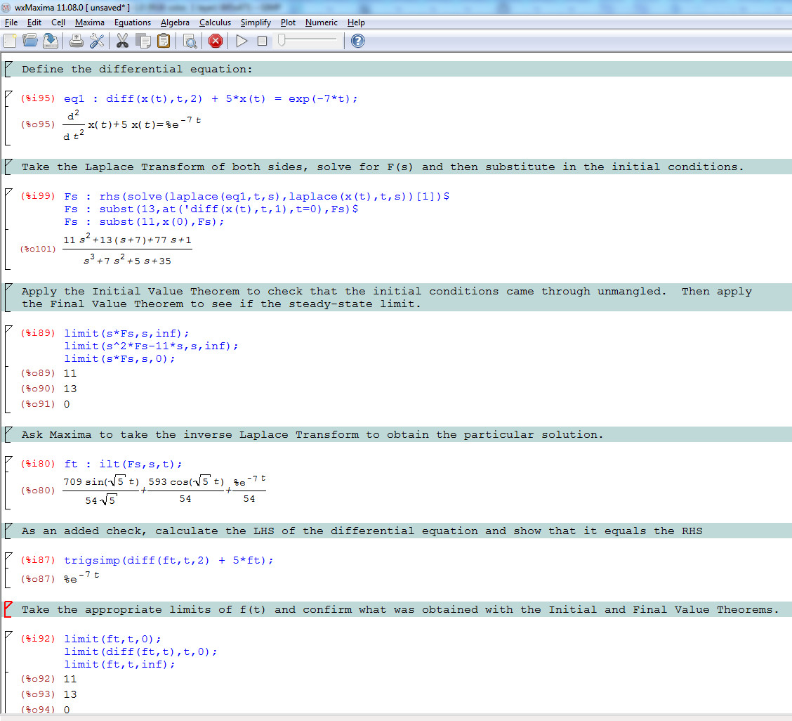
For reference, the wxMaxima steps for this analysis are:
Next week, I’ll be looking at convolution integrals and the products of transforms.