Quantum Evolution – Part 8
In the last two posts, we’ve discussed the path integral and how quantum evolution can be thought of as having contributions from every possible path in space-time such that the sum of their contributions exactly defines the quantum evolution operator $$U$$. In addition, we found that potentials in one dimension of the form $$V = a + b x + c x^2 + d \dot x + e x \dot x$$ kindly cooperate with the evaluation of the path integral. While potentials of these types do lend themselves to problems of both practical and theoretical importance, they exclude one very important class of problems – namely time-dependent potentials. Much of our modern economy is built upon time-dependent electric and magnetic fields, including the imaging sciences of photography and motion pictures, medical and magnetic resonance imaging, microwave ovens, modern electronics, and many more. In this post, I’ll be discussing the general structure for calculating how a quantum state evolves under a time-varying force. The main ingredients in the procedure are the introduction of a new picture, similar to the Schrodinger and Heisenberg pictures, and the perturbative expansion in this picture of the quantum evolution operator.
We start by assuming that the Hamiltonian can be written as
\[ H = H_0 + V(t) \; ,\]
where $$H_0$$ represents the Hamiltonian for some model problem that we can solve exactly. Usually $$H_0$$ represents the free-particle case.
Obviously, the aim is to solve the old and familiar state evolution equation
\[ i \hbar \frac{d}{dt} \left| \psi(t) \right> = H \left| \psi(t) \right> \]
to get the evolution operator that connects the state at the initial time $$t_0$$ with the state at time $$t$$
\[ \left| \psi(t) \right> = U(t,t_0) \left| \psi(t_0) \right> \; .\]
Since we haven’t nailed down any of the attributes of our model Hamiltonian other than it be exactly solvable, I can assume $$H_0 \neq H_0(t)$$. With this assumption, the evolution operator corresponding to $$H_0$$ then
becomes
\[ U_0(t,t_0) = e^{-i H_0(t – t_0)/\hbar} \; , \]
and its inverse is given by the Hermitian conjugate
\[U_0^{-1}(t,t_0) = e^{i H_0(t – t_0)/\hbar} \; .\]
The next step is to introduce a new state $$\left| \lambda (t) \right>$$ defined through the relation
\[ \left| \psi(t) \right> = U_0(t,t_0) \left| \lambda(t) \right> \; .\]
An obvious consequence of the above relation is the boundary condition
\[ \left| \psi(t_0) \right> = \left| \lambda(t_0) \right> \]
when $$t = t_0$$. This relation will come to be useful later.
By introducing this state, we’ve effectively introduced a new picture in which the state kets are defined with respect to a frame that ‘rotates’ in step with the evolution caused by $$H_0$$. This picture is called the Interaction or Dirac picture.
The evolution of this state obeys
\[ \frac{d}{dt} \left| \lambda(t) \right> = \frac{i}{\hbar} H_0 e^{i H_0(t – t_0)/\hbar} \left| \psi(t) \right> + e^{i H_0(t – t_0)/\hbar} \frac{d}{dt} \left| \psi(t) \right> \; , \]
which, when substituting the right-hand side of the time evolution of $$\left| \psi(t) \right>$$, simplifies to
\[ \frac{d}{dt} \left| \lambda(t) \right> = \frac{1}{i\hbar} e^{i H_0(t – t_0)/\hbar} \left[H – H_0\right] \left| \psi(t) \right> \; .\]
The difference between the total and model Hamiltonians is just the time-varying potential and
\[ i \hbar \frac{d}{dt} \left| \lambda(t) \right> = e^{i H_0(t – t_0)/\hbar} V(t) e^{-i H_0(t – t_0)/\hbar} \left| \lambda(t) \right> \equiv V_I(t) \left| \lambda(t) \right> \; , \]
where $$V_I(t) = U_0(t_0,t) V(t) U_0(t,t_0)$$. The ‘I’ subscript indicates that the potential is now specified in the interaction picture. The time evolution of the state $$\left| \lambda(t) \right>$$ leads immediately to the equation of motion
\[ i \hbar \frac{d}{dt} U_I(t,t_0) = V_I(t) U_I(t,t_0) \]
for the evolution operator $$U_I$$ in the interaction picture. The fact that $$U_I$$ evolves only under the action of $$V_I$$ justifies the name ‘interaction picture’.
What to make of the forward and backward propagation in this definition of $$V_I$$? A meaningful interpretation can be made mining the $$U_I$$’s equation of motion as follows.
The formal solution of the equation of motion is
\[ U_I(t,t_0) = Id – \frac{i}{\hbar} \int_{t_0}^t V_I(t’) U(t’,t_0) dt’ \]
but the time dependence of $$V_I$$ means that the iterated solution
\[ U_I(t,t_0) = Id + \sum_{n=1}^{\infty} \left( \frac{-i}{\hbar} \right)^n \int_{t_0}^{t} dt_1 \, \int_{t_0}^{t_1} dt_2 \, … \\ \int_{t_0}^{t_{n-1}} dt_n \, V_I(t_1) V_I(t_2)…V_I(t_n) \]
from case 3 in Part 1 is the only one available.
To understand what’s happening physically, let’s keep terms in this solution only up to $$n=1$$. Doing so yields
\[ U_I(t,t_0) = Id -\frac{i}{\hbar} \int_{t_0}^t \, dt_1 V_I(t_1) \]
or, expanding $$V_I$$ by its definition,
\[ U_I(t,t_0) = Id – \frac{i}{\hbar} \int_{t_0}^t \, dt_1 U_0(t_0,t_1) V(t_1) U(t_1,t_0) \; . \]
From the relationships between $$\left| \psi \right>$$ and $$\left| \lambda \right>$$ we have
\[ \left| \psi(t) \right> = U_0(t,t_0) \left| \lambda(t) \right> = U_0(t,t_0) U_I(t,t_0) \left| \lambda(t_0)\right> \\ = U_0(t,t_0) U_I(t,t_0) \left| \psi(t_0) \right> \]
from which we conclude
Pre-multiplying by the model Hamiltonian’s evolution operator $$U_0$$ gives
\[ U(t,t_0) = U_0(t,t_0) – \frac{i}{\hbar} \int_{t_0}^t \, dt_1 \left( U_0(t,t_0) U_0(t_0,t_1) V(t_1) U(t_1,t_0) \right) \; , \]
which simplifies using the composition property of the evolution operators as
\[ U(t,t_0) = U_0(t,t_0) – \frac{i}{\hbar} \int_{t_0}^t \, dt_1 U_0(t,t_1) V(t_1) U(t_1,t_0) \; .\]
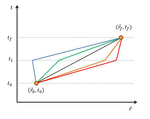
This first-order form for the full evolution operator suggests that its action on a state can be thought of as comprised of two parts. The first part corresponds to the evolution of the state under the action of the model Hamiltonian over the entire time span from $$t_0$$ to $$t$$. The second part corresponds to the evolution of the state by $$U_0$$ from $$t_0$$ to $$t_1$$ at which point the state’s motion is perturbed by $$V(t)$$ and then the state merrily goes on its way under $$U_0$$ from $$t_1$$ to $$t$$. In order to get the correct answer to first order, all intermediate times at which this perturbative interaction can occur must be included. A visual way of representing this description is given by the following figure
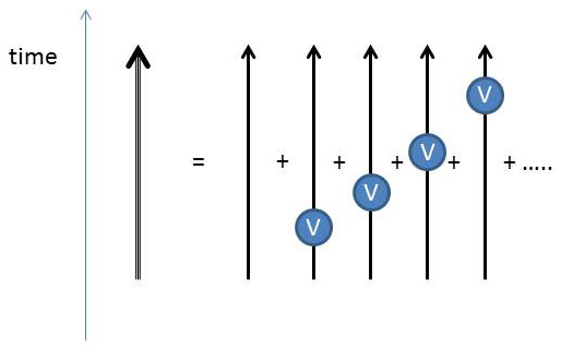
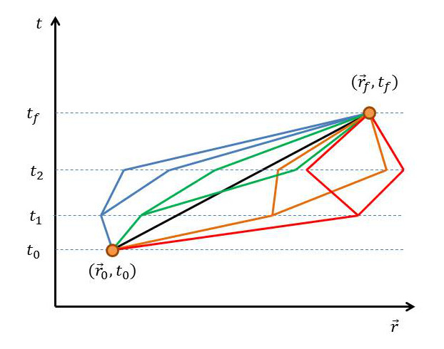
where the thick double line represents the full evolution operator $$U(t,t_0)$$, the thin single line represents the evolution operator $$U_0$$ and the circles represent the interaction with the potential $$V(t)$$ that can happen at any intermediate time. This interpretation can be carried out to any order in the expansion, with two interaction events (two circles) for $$n=2$$, three interaction events (three circles) for $$n=3$$, and so on.
The formal solution of $$U_I$$ can also be manipulated in the same fashion by pre-multiplying by $$U_0$$ to get
\[ U(t,t_0) = U_0(t,t_0) \\ – \frac{i}{\hbar} \int_{t_0}^t \, dt’ U_0(t,t_0) U_0(t_0,t’) V(t’) \; \; U_0(t’,t_0) U_I(t’,t_0) \]
which simplifies to
\[ U(t,t_0) = U_0(t,t_0) – \frac{i}{\hbar} \int_{t_0}^t \, dt’ U_0(t,t’) V(t’) U(t’,t_0) \; . \]
Projecting this equation onto the position basis using $$\left< \vec r \right|$$, $$\left| \vec r_0 \right>$$ and the closure relation $$\int d^3r’ \left| \vec r’ \right>\left< \vec r’\right|$$ for all intermediate positions gives a relationship for the forward-time propagator (Greens Function) of
\[ K^+(\vec r, t; \vec r_0, t_0) = \int_{t_0}^{t} \, dt’ \int \, d^3r’ \\ K^+_0(\vec r, t; \vec r’, t’) V(\vec r’, t’) \; \; K^+(\vec r’, t’; \vec r_0, t_0) \; \]
(compare, e.g., with equation (36.18) in Schiff). This type of analysis leads to the famous Feynman diagrams.