Circular Restricted Three Body Problem – Part 4: Surfaces of Zero Relative Velocity
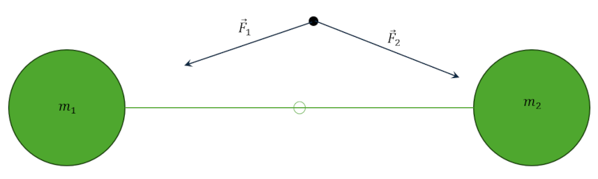
Last month we made a preliminary exploration of the pseudopotential, mapping out the various large-scale features and discovering those characteristics that suggest the basic structure of the 5 equilibrium points. The argument for their existence and their location was made heuristically by appealing to a simple physical problem (two fixed, co-equal masses) that was then ‘relaxed’ into a slightly more complex problem (two co-orbiting, co-equal masses).
This argument is compelling (and correct) and it provides the best guidance for understanding and exploring practical problem. However, it lacks the quantitative aspects required to constructively find the equilibrium points and understand their dynamic stability. Ordinarily this might be viewed as a deficiency that should be immediately remedied (and, in fact, it will be attended to in a sequel) but there is actually a lot more information that can be wrung from this heuristic viewpoint before moving detailed work.
The reason for lingering over these qualitative aspects is that the CRTBP cannot be solved analytically in any meaningful way. Therefore, having qualitative limits on the possible motions is far more important than the usual ones available in the Kepler problem.
For example, energy conservation within the Kepler problem allows us to know that the semi-major axis and the period of resulting elliptical motion is fixed from orbit to orbit. But, this result is not nearly as useful as knowing explicitly that the semi-major axis is given by
\[ a = \frac{ – \mu }{ {\mathcal E} } \; , \]
where ${\mathcal E}$ is the specific energy of motion. In addition, knowing that energy is conserved is not nearly as the vis viva formula for the specific energy
\[ {\mathcal E} = \frac{1}{2} v^2 – \frac{G m}{r} \; , \]
which is the sum of specific kinetic and potential energies. By setting the specific energy to be zero we immediately arrive at the formula for the escape speed from any object, possessing mass $m$, as
\[ v = \sqrt{ \frac{ 2 G m}{r} } \; .\]
These simple relations tell us quite a great deal about the allowed motions in the Kepler problem.
Unfortunately, we can’t make a similar argument in the CRTBP since that dynamical system doesn’t possess a conservation of energy. But it does possess a conserved Jacobi constant and an analogous argument can be made, although it lacks a direct one-to-one interpretation in an important way.
We start with the analog of vis viva in the CRTBP given by the (hopefully) now familiar statement that
\[ v^2 = 2 U – C_J \; . \]
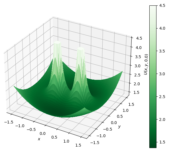
Since the velocity ${\vec v}$ is expressed in the rotating frame, it isn’t directly related to the kinetic energy. Nonetheless, wherever its magnitude becomes zero must be a limit on the spatial excursion of the solutions. By plotting the contours of $U(x,y,z)$ for various values of $C_J$, we can get a visual identification of those regions around the massives where the restricted particle is free to move and of those regions forbidden to it. In the following discussion it is important to remember that, because of the traditional sign convention used in its definition, larger positive values for the Jacobi constant mean that the motion is more tightly bound to one of the two massives.
Obviously in making the requisite contour plots we can use any value of for the mass fraction $\mu$, but, to be concrete, we will be using $\mu = 0.05$ since this value is small enough so that we see behavior similar to what we might see in the solar system but large enough not to pose a challenge in making the plots. For comparison, the Sun-Jupiter mass fraction is around 0.001 while the Earth-Moon mass fraction is approximately 0.01.
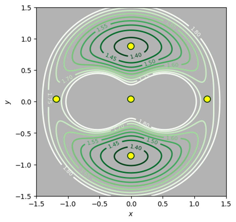
The following figure shows what happens as we lower the value of $C_J$ over the range of values from 6.0 down to 2.9. These values, which are irregularly spaced, were chosen in order to show some prominent features. Regions shaded green are those regions in the $x$-$y$ plane where motion is allowed or, in other words, regions where $U \ge \frac{1}{2} C_J$; gray-shaded regions are forbidden.
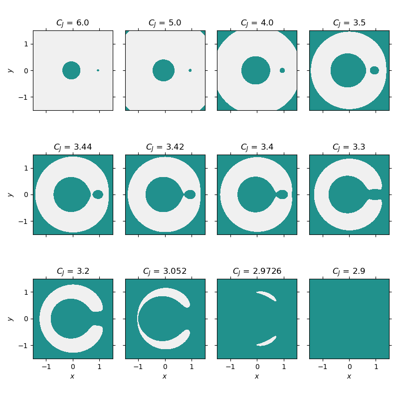
For the initial value of $C_J = 6.0$, we see that particle motion is confined to the vicinity of either the primary (larger, circular region on the left) or to the secondary (smaller circular, region on the right). As the value of $C_J$ shrinks (or, alternatively, as the particle’s motion gets more ‘energetic’), the regions deform and significant bulges appear on the line joining the massives. In addition, regions outside of the massive become accessible as seen by the green corner regions ‘peaking’ into the individual subplots. These regions grow as $C_J$ continues to decrease.
At roughly $C_J = 3.42$ the bulges along the line joining the massives just touch and begin to coalesce. At this point, the restricted body can move from the vicinity of the primary to the secondary and vice versa.
By the time the value of $C_J = 3.3$, a ‘throat’ or ‘gate’ has opened joining the previously inner region around the massives with the outer region. With this configuration, even more exotic motion is possible with the restricted particle being free to move from the vicinity of either the primary or secondary to regions far away and with the ability to return. Of course, nothing in these plots indicate the time required to make the journey – simply that it is possible.
Finally, as the value of $C_J$ gets even smaller, only two regions, roughly near the triangular equilibrium points, remain as forbidden. They persist as forbidden regions until $C_J$ become small enough that they, too, vanish.
While the analogy between $C_J$ and energy is valid, the topological changes that come about indicate that there is something more than strict level surfaces of an energy-like parameter at work. As subsequent posts will show, there is also a component of angular momentum that features in the CRTBP problem in a significant way, partly due to the analysis being done in the rotating frame and partly as a mirror of the importance of angular momentum in the two-body problem. But that is a story for another post.