
The last post introduced the basic model of site percolation in which an $M \times N$ lattice would have each of its sites occupied with a probability $p$. It was demonstrated that by sweeping that probability up through a critical value $p_c$ there was a qualitative change in system. Below $p_c$, there was a small likelihood of finding a spanning cluster, defined as a connected set of sites in which an unbroken path could be made between either the left and right sides of the lattice or the top and bottom of the lattice or both. Above $p_c$ there it is almost certain that a spanning cluster will exist. For a cluster to be connected, nearest neighbor sites must be occupied in the up-down direction or the right-left direction.
The percolation model finds itself in the center of a lot of analysis because it is a simple example of a phase transition, in this case what is known as a geometric phase transition. Phase transitions are familiar in physics and we see numerous examples. Perhaps the most common place one is $H_2 O$ going from solid form (ice) to liquid (water) to gas (steam). Percolation provides a simple playground in which the basic ideas and theoretical foundations can be explored without bringing to account the vast machinery of statistical mechanics. Despite this ‘toy’ status, percolation models are physically interesting in their own way as well.
An enormous amount of work went into understanding how phase transitions occur during the 1960s and 1970s and one of the most celebrated ideas is the notion that the system exhibits a type of length invariance at the transition. The correlation length, properly defined, becomes infinite, and all length scales matter.
In this entry, I’ll try to show what is meant by this notion before turning, in subsequent columns, to the quantitative theory of critical exponents and scaling laws. To this end, the results presented here will be more in the line of a numerical experimentalist presenting the findings of a variety of simulations without the presentation of much in the way of an underlying theory to explain the results from a compact set of premises.
These experiments consisted of running 50 trials of the percolation model for each of 4 lattice sizes: $L = 16$, $32$, $64$, and $128$ cells per linear dimension and over five separate occupation probabilities $p = 0.4$, $0.5$, $0.5927 \equiv p_c$, $0.7$, and $0.8$.
Using the Hoshen-Kopelman cluster identification algorithm, the number of clusters in the lattice were labeled with a unique, sequential cluster id number. These clusters labels afford the ability to both create visual representations of the lattice and perform quantitative analysis.
We’ll start with the visual displays first and only at the end we’ll touch on the quantitative analysis, setting the stage for more detailed discussions in subsequent blogs.
While there are many ways to slice through the various combinations of lattice size and probability, the easiest one to start with is to look how cluster morphology changes as the lattice size changes at a given occupation probability.
For $p = 0.4$, which is well below the critical value $p_c$
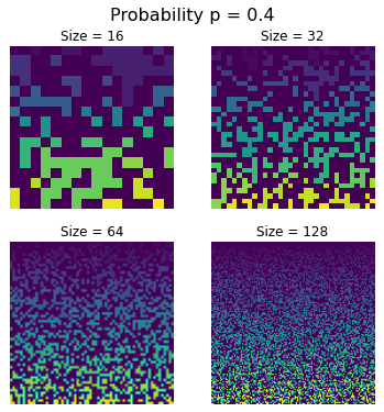
there is a speckling of clusters throughout the whole lattice no matter how big the lattice size. And, as shown last time, the probability of getting a spanning cluster is effectively zero.
Stepping the occupation probability up to the value $p = 0.5$ doesn’t significantly alter anything
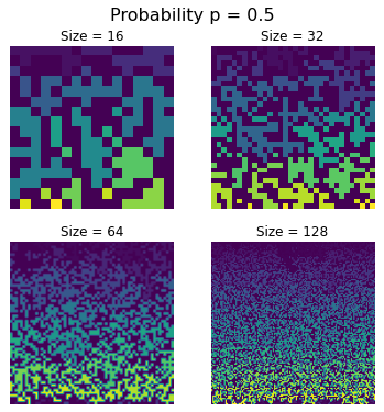
although there are noticeably more clusters albeit somewhat larger ones; the lattices look grainer.
Appearances change remarkably at the critical value $p = p_c = 0.5927$
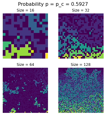
with the clusters both being bigger (each of the examples shown above have a spanning cluster) but also with the clusters being ‘rougher’ and ‘less compact’. Having a way to quantify those observations will be the major focus of the numerical analysis that follows in the months to come.
Raising the occupation probability to $p = 0.7$
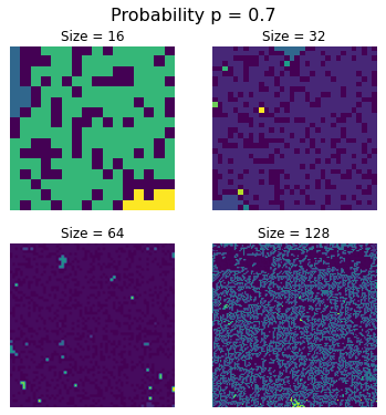
begins eliminating the rougher qualities seen when $p = p_c$ as the spanning cluster effectively crowds out the small clusters as it consumes more and more of the lattice.
By the time $p = 0.8$
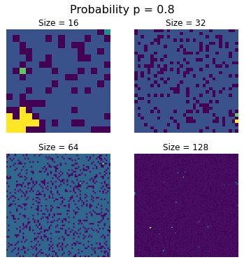
the spanning cluster is leaving very little space for isolated clusters and, effectively, the entire lattice is consumed by a single, connected cluster that reaches all four edges.
It’s clear that at as the occupation probability is driven from low values through $p = p_c$ into high values, that there are three distinct behaviors. When $p << p_c$, the lattice supports small, relatively compact clusters whose presence gives it a rough appearance. When $ p >> p_c$, the lattice is consumed by essentially one large cluster, giving it a smooth or even appearance. At or around $p = p_c$, the lattice seems to have a mix of both small compact clusters and large spanning ones without either behavior dominating. This observation is what is meant by length invariance.
In the months to come, we’ll explore how to quantitatively describe these qualitative observations.