
On the of the most interesting and curious of physical phenomena is the phase transition. We’ve all seen snow and ice melt into water and water boil to steam and then water vapor. The transfer of heat helps materials span the traditional three phases of matter: solid, liquid, and gas. The flow of heat into the system breaks bonds that tend to order the collection of molecules while the flow outward works in the opposite way by ‘slowing motion down’ so that the bonds reestablish.
But the concept of a phase transition is not solely the province of the thermodynamics of physical systems. Any driver of a system that either forces or removes some type of ordering can serve to make a collective exhibit a phase transition.
One of the simplest examples of this latter type is percolation and this blog strongly follows the presentation found in An Introduction to Computer Simulation Methods, Applications to Physical Systems, Vol 2, by Harvey Gould and Jan Tobochnik.
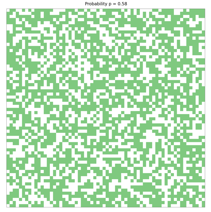
Originally conceived for porous substances, such as rock, the basic idea behind the percolation model on a computer is that there exists a computational lattice with rows and columns of sites that can be empty, denoted with a zero, or occupied, denoted with a one. The lattice is initially unpopulated. Each site is then assigned a random number and if that number is less than some threshold, called the occupation probability, then the site is populated. The figure below shows the result for a 64×64 lattice with the probability set at 0.58.
Up to this point, the algorithm is nothing more than idle play through some basic programming that produces something that might be called computational art. The notion of a phase transition emerges when we ask ourselves what is the likelihood that a spanning cluster emerges in the lattice. A spanning cluster is defined as a set of nearest-neighbor, occupied sites linked together such that they reach across opposite edges of the cluster. A nearest-neighbor linkage occurs when the two occupied sites are either horizontally or vertically adjacent; diagonal linkages do not count.
As example of such a spanning cluster occurs in this next example in which a clearly set of nearest-neighbor linkages running between the bottom and top edges are identified by the black path.
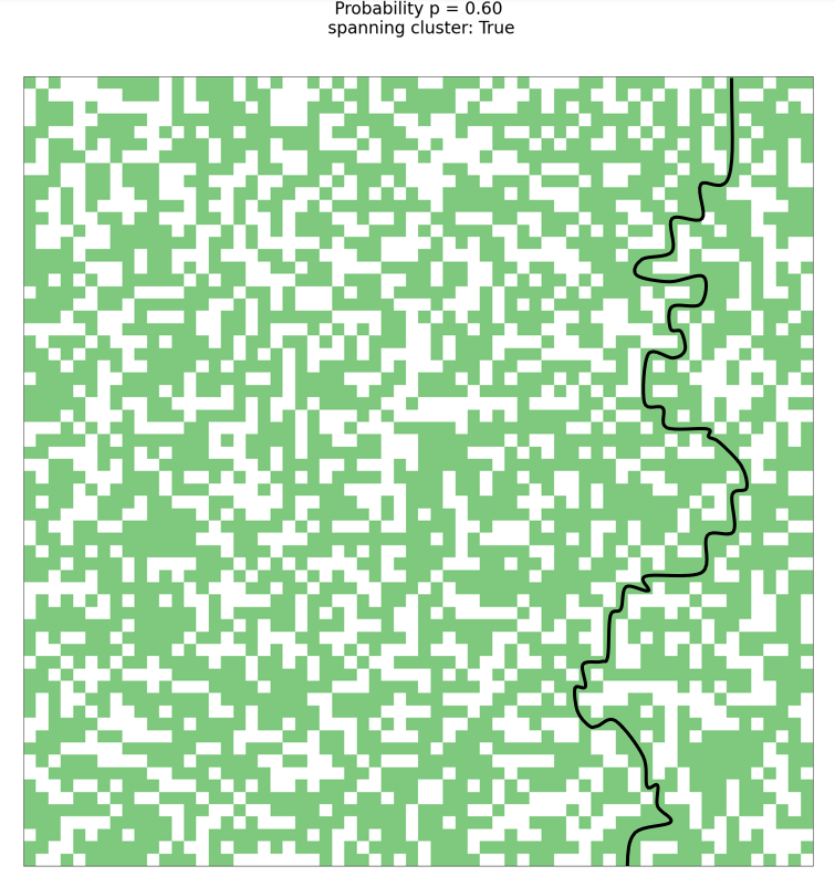
Note that a lattice may exhibit multiple paths linking multiple sites from an edge to its opposite. The only question being asked is whether a path exists not its degeneracy.
To understand how a phase transition might occur, we’ll look at a simple, 8×8 lattice populated with different occupation probabilities and note how often a spanning cluster occurs. To estimate this likelihood, we’ll run 16 separated cases and we’ll count the proportion of these 16 trials that present with a spanning cluster. An 8×8 lattice is chosen both because of the simplicity of finding a spanning cluster by eye but also because it is relatively easy to display all 16 trials simultaneously.
The first set of trials have the occupation probability set to $P = 0.45$
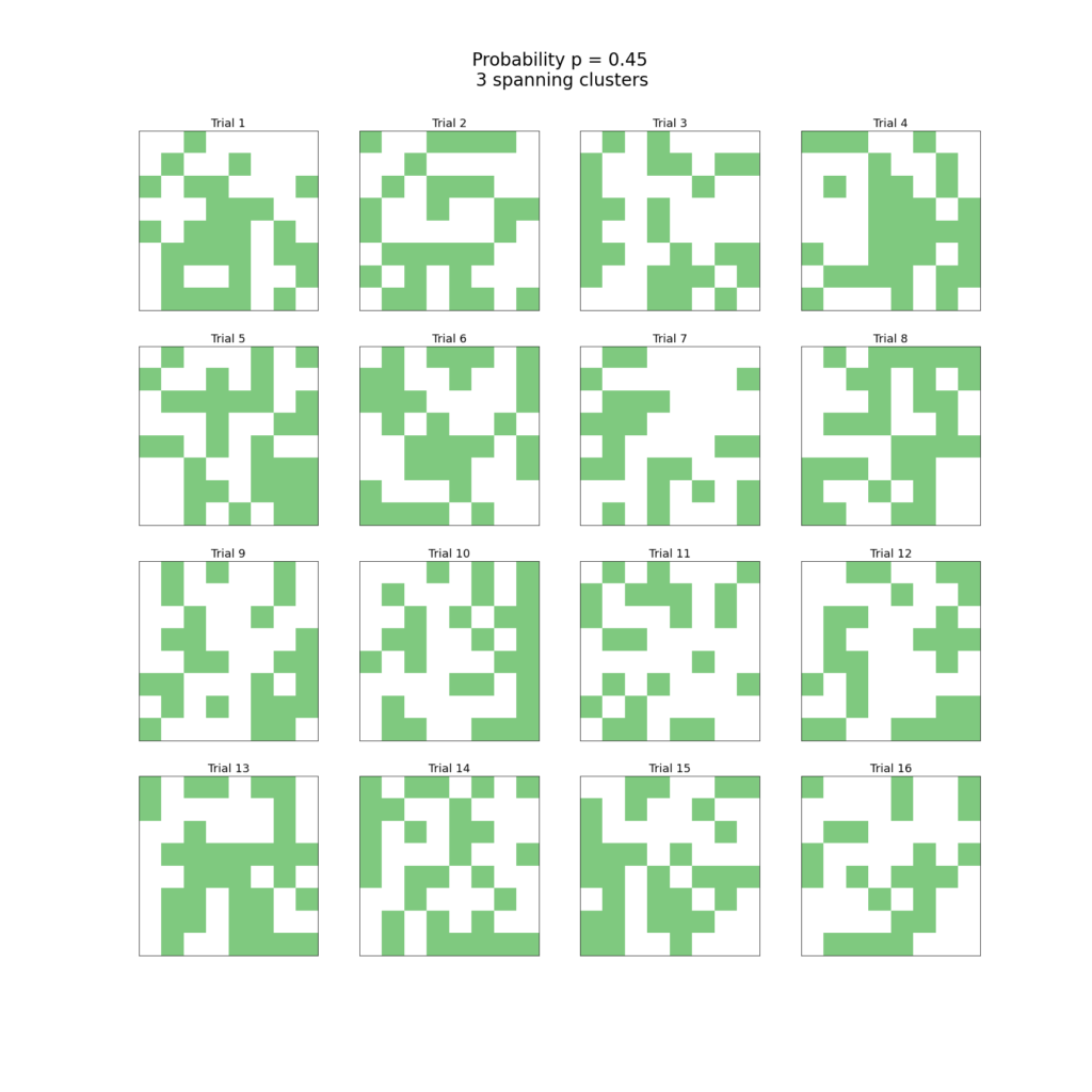
A bit of study should convince us that of the 16 lattices only one exhibited a spanning cluster (3rd row, 2nd column). The remaining lattices got tantalizingly close in some cases (e.g., 1st row, 4th column) but failed to make it all the way across either horizontally or vertically.
For the next set of trials, we set the occupation probability to $P = 0.60$
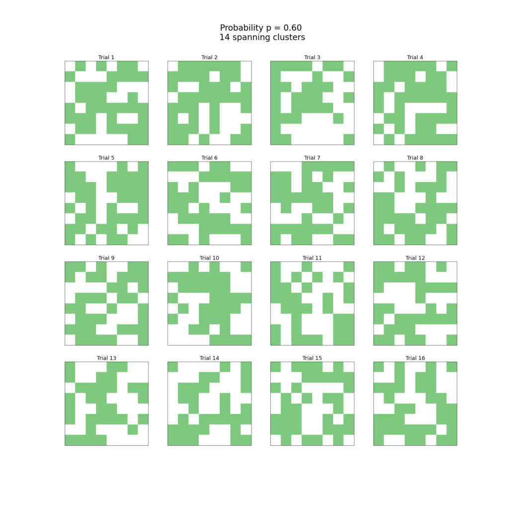
In this scenario, all but two trials had a spanning cluster (3rd row, 1st column and 4th row, 3rd column being the exceptions).
Clearly there is a qualitative change in terms of linkages within the lattice that occurs somewhere between these two values of the occupation probability. And this qualitative change is more than a superficial change in coloration. If these sites represent conducting paths, then electrical current can flow across the lattice when a spanning cluster exists and the lattice transitions from an insulator to a conductor (albeit, perhaps, a poor one). The same holds true with a conventional porous material like rock where now occupation means the absence of material. The presence of a spanning cluster now means that a clear path exists for water to flow through the material (albeit, perhaps, slowly) and the material transitions from one that prevents drainage to one that allows it.
The value we estimate for which this transition takes place between $P = 0.45$ and $P = 0.4$, called the critical occupation probability $P_c$, will generally depend on the size of the lattice. The smaller the lattice, the more likely we are to get a spanning cluster simply as a fluke of statistics whereas for larger lattice sizes events have to transpire just so for a spanning cluster to occur below the critical occupation probability.
The following plot shows the fraction of 16 trials that exhibit a spanning cluster as a function of the occupation probability over the lattice sizes $L = 8, 16, 32, 64$. The Hoshen-Kopleman cluster finding algorithm was used to determine whether a lattice had a spanning cluster automatically.
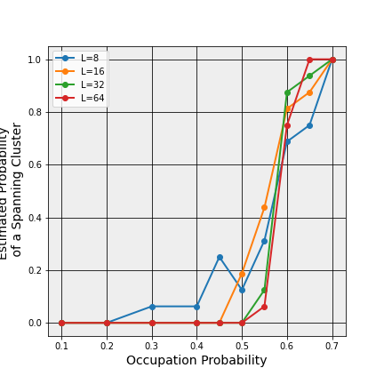
Clearly, there is a remarkably abrupt change in the fraction of trials sporting a spanning cluster at around 0.5 with the sharpness growing as the lattice size $L$ increases. The commonly accepted value for the thermodynamic transition, defined as the value as $L \rightarrow \infty$ is 0.592746.
The value of $P_c$ also depends on the dimension of the system and the topology of the number of nearest neighbors. The following table, adapted from Kim Christensen’s monograph Percolation Theory, shows how the value of $P_c$ changes as a function of dimension and local connectedness.
| Lattice Type | Number of Nearest Neighbors | $P_c$ |
|---|---|---|
| 1D | 2 | 1 |
| 2D Honeycomb | 3 | 0.6962 |
| 2D Square (used above) | 4 | 0.5927 |
| 2D Triangular | 6 | 1/2 |
| 3D Diamond | 4 | 0.4300 |
| 3D Simple Cubic | 6 | 0.3116 |
| 3D Body-Centered Cubic | 8 | 0.2460 |
| 3D Face-Centered Cubic | 12 | 0.1980 |
| 4D Hypercubic | 8 | 0.1970 |
| 5D Hypercubic | 10 | 0.1410 |
| 6D Hypercubic | 12 | 0.1070 |
| 7D Hypercubic | 14 | 0.0890 |
Generally, it holds that as the number of nearest neighbors increases the value of $P_c$ decreases. This is heuristically explained as there are just that many more ways of connecting a spanning path. Also as the number of dimensions increases (even holding the number of nearest neighbors constant) $P_c$ goes down.