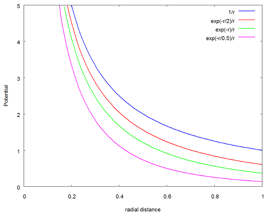
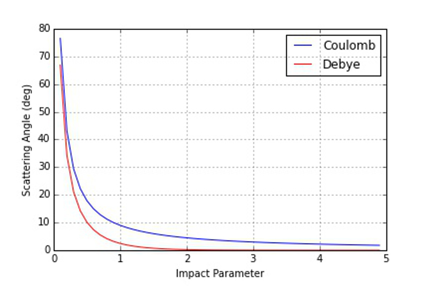
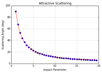
This week’s column is the last installment of a long and detailed look at scattering in classical mechanics. Up to this point specific potentials ($$1/r$$ and $$e^{-r/R}/r$$) have been used and the specific relationship between the impact parameter $$b$$ and the scattering angle $$\theta$$ has been derived either analytically ($$1/r$$) or numerically ($$1/r$$ and $$e^{-r/R}/r$$). This week, I am going to talk about scattering in general and clear up a few loose ends, including a close look at the traditional definition of scattering cross section.

One might argue that the omission of the scattering cross section in these previous studies has been glaring. But as I’ve argued elsewhere, I prefer the definition of the scattering cross section in terms of relative probability and I believe that the insistence on deriving ‘an effective area’ to be a hold over from the pre-quantum days when Rutherford scattering was a new technique and its results were revolutionary. While it is true that scattering results in particle physics still are expressed in barns (or some faction therein), their interpretation is clearly couched in terms of fractions of outcome events compared to all the possible events. In addition, in all my professional work in planetary flybys, I’ve never seen anyone actually calculate a scattering cross section. Rather everything is expressed in terms of impact parameter $$b$$ (from which the b-plane derives its name) and the bend or scattering angle. Even when performing Monte Carlo analysis of flyby control and navigation, no one suggests using cross section. Nonetheless, a really thorough treatment would be incomplete without some discussion.

My treatment here closely follows the arguments found in Chapter 6 of Introduction to Elementary Particles, 2nd edition by David Griffiths. Griffiths doesn’t present anything new, per se, but he is careful in his pedagogy – particularly his ‘derivation’ of $$\frac{d\sigma}{d\Omega}$$ and it is worth extending his approach.

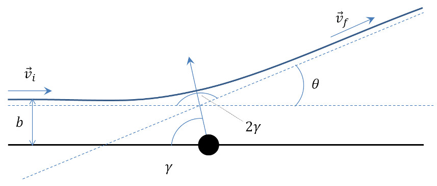
The generic scattering scenario is shown in the figure below.

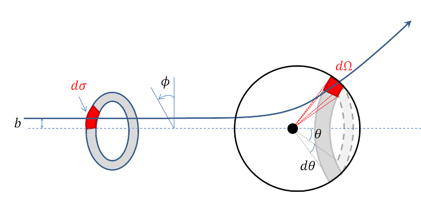
In it, we imagine a uniform and collimated beam of particles streaming towards a scattering center. Focus on one slice through the beam at a point where the particles are still far from the scatterer. Narrow the focus again to those particles in an annular ring with inner radius $$b$$ and outer radius $$b+db$$, denoted by the gray shading. And, finally, narrow the focus one more time to particles in that ring that reside in the sector between azimuth angles $$\phi$$ and $$\phi + d\phi$$. This sector, of area $$d\sigma$$, is denoted by the red shading. As the annular ring propagates towards the scatter, the individual particles begin to be deflected and eventually, when sufficiently long time has passed, the ring will have become distorted into the gray annulus on the sphere surrounding the scatter. In particular, the original red sector has been transformed into a region of solid angle $$d\Omega$$ on the sphere. The (differential) scattering cross section relates the two through

\[ d \sigma = D(\theta,\phi) d \Omega \; .\]

The introduction of $$D(\theta, \phi)$$ by Griffiths is a nice pedagogical touch as it divorces the concept from the stupid notation $$\frac{d\sigma}{d\theta}$$ which is neither explanatory nor actually a derivative in the rigorous sense. By dimensional arguments, $$D(\theta,\phi)$$ must have units of area, a point on which I will elaborate more below.

The area of the sector is

\[ d\sigma = |b \, db \, d\phi| \]

and the solid angle is

\[ d\Omega = |\sin \theta \, d\theta \, d\phi| \; .\]

Note that since area and solid angle are intrinsically positive quantities, whereas $$db$$, $$d\phi$$, and $$d\theta$$ can have any sign, absolute value must be used.

Substituting these relations in and solving for $$D(\theta,\phi)$$ yields

\[ D(\theta,\phi) = \frac{d\sigma}{d\theta} = \frac{|b \, db \, d\phi|}{|\sin \theta \, d\theta \, d\phi|} = \frac{b}{\sin \theta}\left|\frac{db}{d\theta}\right| \; , \]

where $$b$$ and $$\sin\theta$$ can be taken out of the absolute values since they are always positive (since $$b$$ is a radius and $$\sin\theta \ge 0 $$ for $$\theta \in [0,\pi]$$).

So having the relationship between the impact parameter $$b$$ and the scattering angle $$\theta$$ is essentially the same as having the scattering cross section.

For the case of Coloumb scattering, the relationship (as derived in Part 3) is

\[ \cot^2 \left(\frac{\theta}{2}\right) = \frac{4 E^2 b^2}{\alpha^2} \; .\]

To get the scattering cross section, first solve for $$b$$ in terms of $$\theta$$ (note that since we will be taking an absolute value, the sign from the square root doesn’t matter)

\[ b = \frac{\alpha}{2 E} \cot \left( \frac{\theta}{2} \right) \]

and then take the derivative

\[ \left| \frac{db}{d\theta} \right| = \frac{\alpha}{4 E} \csc^2 \left( \frac{\theta}{2} \right) \; . \]

A clever rewriting of $$\sin \theta = 2 \sin\left(\frac{\theta}{2}\right) \cos\left(\frac{\theta}{2}\right)$$ gives

\[ D(\theta,\phi) = \frac{\frac{\alpha}{2E} \frac{\cos\left(\frac{\theta}{2}\right)}{\sin\left(\frac{\theta}{2}\right)}}{2 \sin\left(\frac{\theta}{2}\right) \cos\left(\frac{\theta}{2}\right)} \cdot \frac{\alpha}{4 E} \frac{1}{\sin^2\left(\frac{\theta}{2}\right)} = \; \; \; \frac{1}{4} \left(\frac{\alpha}{2E}\right)^2 \csc^4 \left( \frac{\theta}{2} \right) \; ,\]

which is the famous Rutherford result.

Physically, from the defining equation, $$D(\theta,\phi) d\Omega$$ is the area of the image of the incoming red sector under the action of the scattering. It is often expressed as

\[ D(\theta,\phi) d\Omega = \frac{\textrm{# of particles per unit time scattered into } d \Omega}{\textrm{incident intensity}} \; . \]

To see why, suppose that the incident intensity $$I_0$$ is given by

\[ I_0 = \frac{N}{A \delta t} \; ,\]

where $$N$$ is the number of particles in the beam, $$A$$ is the cross sectional area of the beam, and $$\delta t$$ is some measure of unit time. Let $$N_{d\Omega}$$ be the number of particles scattered in solid angle $$d\Omega$$. The unit of time cancels leaving

\[ D(\theta,\phi) d\Omega = A \frac{N_{d\Omega}}{N} \; ; \]

so, like in the Monte Carlo case discussed earlier, the area of the image can be inferred by counting how many particles end up in it relative to the number of particles sent in and multiplying the initial area of the beam by this scale factor. For those needing a bit more convincing, realize that the number of scattered particles $$N_{d\Omega}$$ is equal to the number of particles in the original red sector (this is a classical setting to local neighborhoods propagate into local neighborhoods). The number of particles in the original red sector is the fraction of cross sectional area it consumes times the total number or

\[ N_{d\Omega} = N_{d\sigma} = N \frac{d\sigma}{A} \; ,\]

which when substituted into the previous equation gives $$D(\theta,\phi) d \Omega = d\sigma$$ as desired. The experimentalist is likely to massage these last relationship into a pithier statement: $$D(\theta,\phi) d\Omega = N_{d\Omega} / I_0$$ (the cross section equals the particles counted divided by the beam intensity).

Nowhere in any of the above discussion is there an interpretation that says that $$D(\theta,\phi) d\Omega$$ is somehow the size of the scatterer. In fact, if one defines, the size of the scatter as

\[ S = \int d\Omega D(\theta,\phi) \]

then one is baffled by the result that, for Coloumb scattering, the size of the scatterer is infinite. Bigger than the experiment, bigger than the universe, and certainly so big as to thwart every assumption we have about incoming and outgoing unbound states. This is the heart of my objection to that interpretation.

So from where does such an interpretation spring? Well, in one particular case – and only in this case – does it make some kind of sense. For scattering from a hard sphere

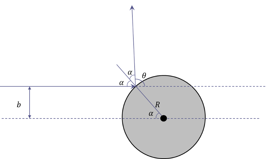
the relationship between the impact parameter and the scattering angle (which can be read off from the above geometry) is

\[ b = R \cos\left(\frac{\theta}{2}\right) \; . \]

The derivative, which is very easy to compute, is

\[ \frac{db}{d\theta} = -\frac{R}{2} \sin\left(\frac{\theta}{2}\right) \; \]

and

\[ D(\theta,\phi) = \frac{R^2}{4} \; .\]

Integrating this expression over the entire solid angle gives

\[ \int d\Omega D(\theta,\phi) = \pi R^2 \; .\]

Certainly interesting and encouraging, but totally misleading, since the ‘potential’ for hard sphere scattering has compact support, a situation that most potentials of interest fail to possess.

In last week’s column, the relationship between the impact parameter and the scattering angle for a $$1/r$$ potential was examined in some detail for both attractive and repulsive scattering. The excellent agreement between theory and the numerical simulations was evident in how well the energy, angular momentum, and eccentricity vector were conserved and in how accurately the observed scattering angle matched the predicted functional form as a function of impact parameter.

This week, the picture changes somewhat as the $$e^{-r}/r$$ potential replaces the $$1/r$$ potential. In addition, the coupling constant $$\alpha$$ will always be negative so that repulsive scattering results in both cases for easy comparison. For convenience, the $$1/r$$ case will be referred to as Coulomb scattering. Although a genuine argument can be made for Rutherford scattering as the proper name, based on the his historic experiments, I use Coulomb since the resulting force comes from Coulomb’s law.

The new force law is dubbed Debye since it is functionally identical to the force that results from Debye shielding in a plasma. The full form of the potential is

\[ \frac{\alpha e^{-r/R}}{r} \; , \]

where $$R$$ sets the scale length of the potential. The corresponding Debye equation of motion is

\[ \ddot {\vec r} + \frac{\alpha (R+r) e^{-r/R} }{R r^3} \vec r = 0 \; .\]

Since the Debye force is central and time-invariant, angular momentum and energy are conserved. The eccentricity vector, which is properly a quantity only for conic sections, is not used in the Debye case. Most likely there isn’t an additional conserved quantity that is it’s analog for Debye scattering. This conclusion is based on Betrand’s Theorem, which says that only $$1/r$$ and $$r^2$$ potentials have bound orbits which close (i.e. have a conserved eccentricity vector). Since the derivation that gave the conservation of $$\vec e$$ in the Coulomb case did not depend on the orbits being bound, the obvious conclusion is that an additional conserved quantity on par with the eccentricity vector doesn’t exist for $$e^{-r}/r$$ potentials. In any event, it was only used to get the radial equation and then to subsequently derive an analytical expression that relates the scattering angle $$\theta$$ to the impact parameter $$b$$. Numerical simulations will serve just as well in this case.

Before simulating the scattering, it is helpful to have an expectation as to the general qualitative results. The figure below shows a comparison between the Coloumb and Debye potentials near the scattering center. Note that three separate values of $$R = 2, 1, 1/2$$ are displayed.

In all cases, the Debye potential is below the Coulomb potential, sometimes substantially so. As $$R$$ increases, the Debye ppotential uniformly approaches the Coulomb potential and in the limit as $$R \rightarrow \infty$$, they become the same.

As before, all the numeric simulation were performed using numpy, scipy, and matplotlib within the Jupyter framework. The right-hand-side (RHS) of the equations of motion was computed from

def Debye(state,t,params):
    #unpack the state
    x     = state[0]
    y     = state[1]
    z     = state[2]
    vx    = state[3]
    vy    = state[4]
    vz    = state[5]
    
    #unpack params
    alpha = params['alpha']
    R     = params['R']
    
    #define helpers
    r     = sp.sqrt(x**2 + y**2 + z**2)
    q     = alpha*(r+R)*sp.exp(-r/R)/r**3/R
    
    #state derive
    ds = [vx, vy, vz, -q*x, -q*y, -q*z]
    return ds

Note the implicit understanding that the python dictionary params is now carrying the values of two simulation constants: $$\alpha$$ and $$R$$.

Since the force was derived from a potential, the form of the conserved energy for Debye scattering is

\[ E = \frac{1}{2} v^2 – \frac{\alpha e^{-r/R}}{r} \; .\]

As a check on the accuracy of the simulation, a specific scattering case was examined in detail for both the Debye and Coulomb cases. The initial conditions were

\[ \bar S = \left[ \begin{array}{c} -30 \\ 0.1 \\ 0 \\ 2.25 \\ 0 \\ 0 \end{array} \right] \; .\]

The results for the conserved energy and angular momentum, shown in the figure below, indicate excellent behavior from the numerical simulation.

For comparison, the resulting conservation accuracy in the Coloumb case, shown below, is essentially the same.

Based on the qualitative analysis of the potentials, we expect to see that Debye scattering gets closer to the scattering center and is deflected less than Coulomb scattering, all other things remaining the same. This is exactly what is observed.

With these initial validations done, the final step is to scan over a variety of impact parameters and then to compare the behavior of the scattering angle in the two cases. The same scan_impact_param function was used as in the last post with one modification. The calling sequence was modified to take an additional argument called model, which is a function pointer to the desired RHS of the equation of motion.

def scan_impact_param(b_range,s0,params,model):
    theta              = b_range[:]*0.0
    counter            = 0
    for b in b_range:
        timespan       = np.arange(0,20,0.001)
        s0[1]          = b
        soln           = ode(model,s0,timespan,args=(params,),rtol=1e-8,atol=1e-10)
        theta[counter] = scattering_angle(soln)
        counter        = counter + 1
    return theta

The resulting scattering plot shows, as expected, that the Debye potential allows the scattered particle closer access to the scattering center for a given scattering angle than does the Coulomb potential.

Next week, I’ll tidy up some odds and ends and close out this revisit of classical scattering.

The last post presented the basic methods for numerically integrating a scattering trajectory in a $$1/r$$ potential and demonstrated the excellent agreement between the theoretically-derived conserved quantities and the numerically generated ephemerides. In addition, the point of closest approach predicted from the radial equation agreed to a high degree of precision with what was seen in the integrated trajectories.

This installment extends these techniques to an ensemble of trajectories and, in doing so, allows for the same kind of validation of the scattering cross section predicted by the theory with those obtained from the simulated trajectories.

The theoretical results will be obtained from an careful analysis of the radial equation and the adoption of the usual definitions that related the impact parameter $$b$$ with the outgoing scattered angle $$\theta$$. The simulation results come from routines that scan over values of the impact parameter, produce the corresponding simulated trajectory, and then determine the scattering angle. As in last week’s post, all the numerical modeling is done using Python 2.7 with numpy, scipy, and matplotlib.

The figure below shows an ensemble of scattering trajectories, all having the same energy, that differ only in the perpendicular distance, called the impact parameter $$b$$, from the scattering center.

The smaller values of $$b$$ have the much larger deflection and the variation as the impact parameter is changed clearly not linear. The scattering geometry for an arbitrary trajectory is shown here

The scattering angle $$\theta$$, obviously a function of impact parameter $$b$$, is what we are looking to obtain. Three separate pieces are need to derive a relationship between the scattering angle and the impact parameter:

1. relate the impact parameter to the angular momentum and energy
2. relate the eccentricity to the angular momentum and energy
3. relate the scattering angle to the eccentricity

The first and third relationships are relatively easy but the second requires some work. Let’s take them in order.

Impact Parameter, Angular Momentum, and Energy

Note that far from the scattering center ($$r \rightarrow \infty$$), the incoming velocity $$\vec v_i$$ is perpendicular to the perpendicular distance of the incoming asymptote from the scattering center. This latter term has a magnitude $$b$$ and thus the magnitude of the angular momentum is

\[ L = b v_i \; . \]

At an infinite distance from the scattering center, the potential energy contributes nothing, and the energy is given by

\[ E = \frac{1}{2} v_i^2 \; .\]

Eccentricity, Angular Momentum, and Energy

Relating impact parameter to the angular momentum and the energy is best done by working with a periapis. While there is way to handle both repulsive and attractive scattering on the same footing, it is easier to take them one at a time. Nonetheless, the formula that obtains in both cases is the same.

For repulsive scattering, the radius and the speed at periapis become

\[ r_p = \frac{p}{e-1} = -\frac{L^2}{\alpha (e-1) } \; ,\]

(since $$p=-L^2/\alpha$$), and

\[ v_p = \frac{L}{r_p} = -\frac{\alpha}{L}(e-1) \; .\]

Plugging both of these into the energy gives the expression

\[ E = \frac{1}{2} \frac{\alpha^2}{L^2} (e-1)^2 – \frac{\alpha}{-L^2/\alpha} (e-1) \; .\]

Expanding and simplifying results in

\[ \frac{2 E L^2}{\alpha^2} = e^2 – 1 \]

or, as it is more usually expressed

\[ e = \sqrt{1 + \frac{2 E L^2}{\alpha^2} } \; .\]

Following similar lines, the radius and speed at periapsis for attractive scattering are

\[ r_p = \frac{p}{1+e} = \frac{L^2}{ \alpha (1+e) } \; , \]

(since $$p = L^2/\alpha$$), and

\[ v_p = \frac{\alpha}{L} (1+e) \; .\]

Again plugging these into the energy equation is the next step, which gives

\[ E = \frac{1}{2} \frac{\alpha^2}{L^2} (1+e)^2 – \frac{\alpha^2}{L^2}(1+e) \; .\]

Expanding and simplifying results in exactly the same expression as above. This seemingly coincidental good fortune is a consequence of the underlying conic section properties of these hyperbolic orbit.

Scattering angle and eccentricity

The condition for starting far from the scattering center such that $$r \rightarrow \infty$$ requires that the denominator of the radial equation tend to zero. Taking that limit yields

\[ e \cos \gamma – 1 = 0 \; ,\]

for repulsive scattering, and

\[ 1 + e \cos \gamma = 0 \; , \]

for attractive scattering. The angle $$2 \gamma$$ is often referred to as the bend angle for attractive scattering (for example in analyzing planetary flybys). The relationship between the half-bend angle $$\gamma$$ and the scattering angle $$\theta$$ is

\[ 2 \gamma + \theta = \pi \]

as can be determined, by inspection, from the scattering geometry figure above.

For repulsive scattering,

\[ \cos \gamma = \cos \left(\frac{\pi}{2} – \frac{\theta}{2} \right) = \sin\left(\frac{\theta}{2} \right) = \frac{1}{e} \;. \]

For attractive scattering,

\[ \cos \gamma = \cos \left( \frac{\pi}{2} – \frac{\theta}{2} \right) = \sin \left(\frac{\theta}{2}\right) = -\frac{1}{e} \; .\]

Now we are in position to combine all these ingredients together to get the desired relationship.

Substituting the initial conditions $$E = \frac{1}{2} v_i^2$$ and $$L = b v_i$$ into the eccentricity-angular-momentum-energy relation gives

\[ e^2 = 1 + \frac{2 E b^2 v_i^2}{\alpha^2} = 1+ \frac{4 E b^2 \left( \frac{1}{2} v_i^2\right)}{\alpha^2} = 1 + \frac{4 E^2 b^2}{\alpha^2} \; . \]

Eliminating $$e$$ in favor of the scattering angle $$\theta$$ yields

\[ \frac{1}{\sin^2\left(\frac{\theta}{2}\right)} = 1 + \frac{4 E^2 b^2}{\alpha^2} \; ,\]

where the sign difference between the two types of scattering is now lost since the key relationship involves $$e^2$$.

Using standard trigonometric relations yields the traditional expression

In order to test this expression, two new functions were added to the Python suite of tools. The first is function that takes the ephemeris and calculates the approximate scattering angle by taking the dot product between the first and last velocities. Note the careful avoidance of calling them either the initial or final velocities as there is no practical way to start or finish an infinite distance away.

def scattering_angle(soln):
    vi     = soln[0,3:6]
    vf     = soln[max(soln.shape)-1,3:6]
    vi_mag = sp.sqrt( vi[0]**2 + vi[1]**2 + vi[2]**2 )
    vf_mag = sp.sqrt( vf[0]**2 + vf[1]**2 + vi[2]**2 )
    vdot   = vi[0]*vf[0] + vi[1]*vf[1] + vi[2]*vf[2]
    theta = sp.arccos(vdot/vi_mag/vf_mag)
    return theta

The second function scans over a range of impact parameters and returns the scattering angle for each value.

def scan_impact_param(b_range,s0,params):
    theta              = b_range[:]*0.0
    counter            = 0
    for b in b_range:
        timespan       = np.arange(0,60*200,30)
        s0[1]          = b
        soln           = ode(TwoBody,s0,timespan,args=(params,),rtol=1e-8,atol=1e-10)
        theta[counter] = scattering_angle(soln)
        counter        = counter + 1
    return theta

Taken together, they comprise the ‘experimental’ measurements for these simulations.

Running these for repulsive scattering gives excellent agreement between theory (red line) and experiment (blue dots).

Likewise, similarly excellent agreement is obtained between theory (red line) and experiment (blue dots) for attractive scattering.

Note that the difference between the two plots is attributable to the fact that the same initial conditions (except for the value of $$b$$) were used in both simulations. This was done for convenience. In sign difference in the potential results in higher energy scattering in the repulsive case compared to the attractive and this is why the attractive scattering is slightly more pronounced.

Now that we are sure that our relationship between $$b$$ and $$\theta$$ is correct, we can derive the differential scattering cross section. This will be covered in detail in next week’s installment.