
The last post presented the basic methods for numerically integrating a scattering trajectory in a $$1/r$$ potential and demonstrated the excellent agreement between the theoretically-derived conserved quantities and the numerically generated ephemerides. In addition, the point of closest approach predicted from the radial equation agreed to a high degree of precision with what was seen in the integrated trajectories.
This installment extends these techniques to an ensemble of trajectories and, in doing so, allows for the same kind of validation of the scattering cross section predicted by the theory with those obtained from the simulated trajectories.
The theoretical results will be obtained from an careful analysis of the radial equation and the adoption of the usual definitions that related the impact parameter $$b$$ with the outgoing scattered angle $$\theta$$. The simulation results come from routines that scan over values of the impact parameter, produce the corresponding simulated trajectory, and then determine the scattering angle. As in last week’s post, all the numerical modeling is done using Python 2.7 with numpy, scipy, and matplotlib.
The figure below shows an ensemble of scattering trajectories, all having the same energy, that differ only in the perpendicular distance, called the impact parameter $$b$$, from the scattering center.
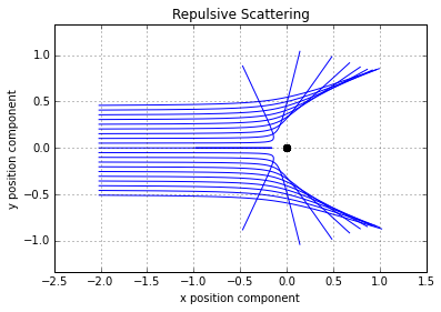
The smaller values of $$b$$ have the much larger deflection and the variation as the impact parameter is changed clearly not linear. The scattering geometry for an arbitrary trajectory is shown here
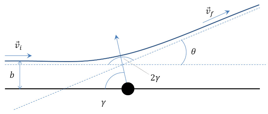
The scattering angle $$\theta$$, obviously a function of impact parameter $$b$$, is what we are looking to obtain. Three separate pieces are need to derive a relationship between the scattering angle and the impact parameter:
- relate the impact parameter to the angular momentum and energy
- relate the eccentricity to the angular momentum and energy
- relate the scattering angle to the eccentricity
The first and third relationships are relatively easy but the second requires some work. Let’s take them in order.
Impact Parameter, Angular Momentum, and Energy
Note that far from the scattering center ($$r \rightarrow \infty$$), the incoming velocity $$\vec v_i$$ is perpendicular to the perpendicular distance of the incoming asymptote from the scattering center. This latter term has a magnitude $$b$$ and thus the magnitude of the angular momentum is
\[ L = b v_i \; . \]
At an infinite distance from the scattering center, the potential energy contributes nothing, and the energy is given by
\[ E = \frac{1}{2} v_i^2 \; .\]
Eccentricity, Angular Momentum, and Energy
Relating impact parameter to the angular momentum and the energy is best done by working with a periapis. While there is way to handle both repulsive and attractive scattering on the same footing, it is easier to take them one at a time. Nonetheless, the formula that obtains in both cases is the same.
For repulsive scattering, the radius and the speed at periapis become
\[ r_p = \frac{p}{e-1} = -\frac{L^2}{\alpha (e-1) } \; ,\]
(since $$p=-L^2/\alpha$$), and
\[ v_p = \frac{L}{r_p} = -\frac{\alpha}{L}(e-1) \; .\]
Plugging both of these into the energy gives the expression
\[ E = \frac{1}{2} \frac{\alpha^2}{L^2} (e-1)^2 – \frac{\alpha}{-L^2/\alpha} (e-1) \; .\]
Expanding and simplifying results in
\[ \frac{2 E L^2}{\alpha^2} = e^2 – 1 \]
or, as it is more usually expressed
\[ e = \sqrt{1 + \frac{2 E L^2}{\alpha^2} } \; .\]
Following similar lines, the radius and speed at periapsis for attractive scattering are
\[ r_p = \frac{p}{1+e} = \frac{L^2}{ \alpha (1+e) } \; , \]
(since $$p = L^2/\alpha$$), and
\[ v_p = \frac{\alpha}{L} (1+e) \; .\]
Again plugging these into the energy equation is the next step, which gives
\[ E = \frac{1}{2} \frac{\alpha^2}{L^2} (1+e)^2 – \frac{\alpha^2}{L^2}(1+e) \; .\]
Expanding and simplifying results in exactly the same expression as above. This seemingly coincidental good fortune is a consequence of the underlying conic section properties of these hyperbolic orbit.
Scattering angle and eccentricity
The condition for starting far from the scattering center such that $$r \rightarrow \infty$$ requires that the denominator of the radial equation tend to zero. Taking that limit yields
\[ e \cos \gamma – 1 = 0 \; ,\]
for repulsive scattering, and
\[ 1 + e \cos \gamma = 0 \; , \]
for attractive scattering. The angle $$2 \gamma$$ is often referred to as the bend angle for attractive scattering (for example in analyzing planetary flybys). The relationship between the half-bend angle $$\gamma$$ and the scattering angle $$\theta$$ is
\[ 2 \gamma + \theta = \pi \]
as can be determined, by inspection, from the scattering geometry figure above.
For repulsive scattering,
\[ \cos \gamma = \cos \left(\frac{\pi}{2} – \frac{\theta}{2} \right) = \sin\left(\frac{\theta}{2} \right) = \frac{1}{e} \;. \]
For attractive scattering,
\[ \cos \gamma = \cos \left( \frac{\pi}{2} – \frac{\theta}{2} \right) = \sin \left(\frac{\theta}{2}\right) = -\frac{1}{e} \; .\]
Now we are in position to combine all these ingredients together to get the desired relationship.
Substituting the initial conditions $$E = \frac{1}{2} v_i^2$$ and $$L = b v_i$$ into the eccentricity-angular-momentum-energy relation gives
\[ e^2 = 1 + \frac{2 E b^2 v_i^2}{\alpha^2} = 1+ \frac{4 E b^2 \left( \frac{1}{2} v_i^2\right)}{\alpha^2} = 1 + \frac{4 E^2 b^2}{\alpha^2} \; . \]
Eliminating $$e$$ in favor of the scattering angle $$\theta$$ yields
\[ \frac{1}{\sin^2\left(\frac{\theta}{2}\right)} = 1 + \frac{4 E^2 b^2}{\alpha^2} \; ,\]
where the sign difference between the two types of scattering is now lost since the key relationship involves $$e^2$$.
Using standard trigonometric relations yields the traditional expression
In order to test this expression, two new functions were added to the Python suite of tools. The first is function that takes the ephemeris and calculates the approximate scattering angle by taking the dot product between the first and last velocities. Note the careful avoidance of calling them either the initial or final velocities as there is no practical way to start or finish an infinite distance away.
def scattering_angle(soln):
    vi     = soln[0,3:6]
    vf     = soln[max(soln.shape)-1,3:6]
    vi_mag = sp.sqrt( vi[0]**2 + vi[1]**2 + vi[2]**2 )
    vf_mag = sp.sqrt( vf[0]**2 + vf[1]**2 + vi[2]**2 )
    vdot   = vi[0]*vf[0] + vi[1]*vf[1] + vi[2]*vf[2]
    theta = sp.arccos(vdot/vi_mag/vf_mag)
    return theta
The second function scans over a range of impact parameters and returns the scattering angle for each value.
def scan_impact_param(b_range,s0,params):
    theta              = b_range[:]*0.0
    counter            = 0
    for b in b_range:
        timespan       = np.arange(0,60*200,30)
        s0[1]          = b
        soln           = ode(TwoBody,s0,timespan,args=(params,),rtol=1e-8,atol=1e-10)
        theta[counter] = scattering_angle(soln)
        counter        = counter + 1
    return theta
Taken together, they comprise the ‘experimental’ measurements for these simulations.
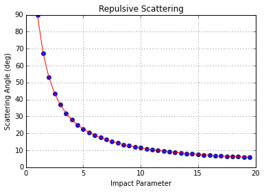
Running these for repulsive scattering gives excellent agreement between theory (red line) and experiment (blue dots).
Likewise, similarly excellent agreement is obtained between theory (red line) and experiment (blue dots) for attractive scattering.
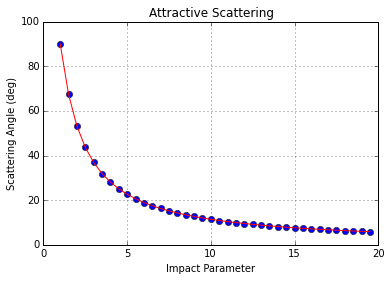
Note that the difference between the two plots is attributable to the fact that the same initial conditions (except for the value of $$b$$) were used in both simulations. This was done for convenience. In sign difference in the potential results in higher energy scattering in the repulsive case compared to the attractive and this is why the attractive scattering is slightly more pronounced.
Now that we are sure that our relationship between $$b$$ and $$\theta$$ is correct, we can derive the differential scattering cross section. This will be covered in detail in next week’s installment.