
In last week’s column, the relationship between the impact parameter and the scattering angle for a $$1/r$$ potential was examined in some detail for both attractive and repulsive scattering. The excellent agreement between theory and the numerical simulations was evident in how well the energy, angular momentum, and eccentricity vector were conserved and in how accurately the observed scattering angle matched the predicted functional form as a function of impact parameter.
This week, the picture changes somewhat as the $$e^{-r}/r$$ potential replaces the $$1/r$$ potential. In addition, the coupling constant $$\alpha$$ will always be negative so that repulsive scattering results in both cases for easy comparison. For convenience, the $$1/r$$ case will be referred to as Coulomb scattering. Although a genuine argument can be made for Rutherford scattering as the proper name, based on the his historic experiments, I use Coulomb since the resulting force comes from Coulomb’s law.
The new force law is dubbed Debye since it is functionally identical to the force that results from Debye shielding in a plasma. The full form of the potential is
\[ \frac{\alpha e^{-r/R}}{r} \; , \]
where $$R$$ sets the scale length of the potential. The corresponding Debye equation of motion is
\[ \ddot {\vec r} + \frac{\alpha (R+r) e^{-r/R} }{R r^3} \vec r = 0 \; .\]
Since the Debye force is central and time-invariant, angular momentum and energy are conserved. The eccentricity vector, which is properly a quantity only for conic sections, is not used in the Debye case. Most likely there isn’t an additional conserved quantity that is it’s analog for Debye scattering. This conclusion is based on Betrand’s Theorem, which says that only $$1/r$$ and $$r^2$$ potentials have bound orbits which close (i.e. have a conserved eccentricity vector). Since the derivation that gave the conservation of $$\vec e$$ in the Coulomb case did not depend on the orbits being bound, the obvious conclusion is that an additional conserved quantity on par with the eccentricity vector doesn’t exist for $$e^{-r}/r$$ potentials. In any event, it was only used to get the radial equation and then to subsequently derive an analytical expression that relates the scattering angle $$\theta$$ to the impact parameter $$b$$. Numerical simulations will serve just as well in this case.
Before simulating the scattering, it is helpful to have an expectation as to the general qualitative results. The figure below shows a comparison between the Coloumb and Debye potentials near the scattering center. Note that three separate values of $$R = 2, 1, 1/2$$ are displayed.
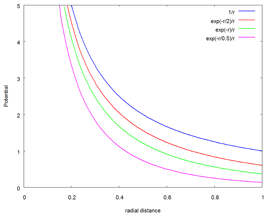
In all cases, the Debye potential is below the Coulomb potential, sometimes substantially so. As $$R$$ increases, the Debye ppotential uniformly approaches the Coulomb potential and in the limit as $$R \rightarrow \infty$$, they become the same.
As before, all the numeric simulation were performed using numpy, scipy, and matplotlib within the Jupyter framework. The right-hand-side (RHS) of the equations of motion was computed from
def Debye(state,t,params):
    #unpack the state
    x     = state[0]
    y     = state[1]
    z     = state[2]
    vx    = state[3]
    vy    = state[4]
    vz    = state[5]

    #unpack params
    alpha = params['alpha']
    R     = params['R']

    #define helpers
    r     = sp.sqrt(x**2 + y**2 + z**2)
    q     = alpha*(r+R)*sp.exp(-r/R)/r**3/R

    #state derive
    ds = [vx, vy, vz, -q*x, -q*y, -q*z]
    return ds
Note the implicit understanding that the python dictionary params is now carrying the values of two simulation constants: $$\alpha$$ and $$R$$.
Since the force was derived from a potential, the form of the conserved energy for Debye scattering is
\[ E = \frac{1}{2} v^2 – \frac{\alpha e^{-r/R}}{r} \; .\]
As a check on the accuracy of the simulation, a specific scattering case was examined in detail for both the Debye and Coulomb cases. The initial conditions were
\[ \bar S = \left[ \begin{array}{c} -30 \\ 0.1 \\ 0 \\ 2.25 \\ 0 \\ 0 \end{array} \right] \; .\]
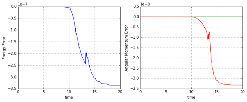
The results for the conserved energy and angular momentum, shown in the figure below, indicate excellent behavior from the numerical simulation.
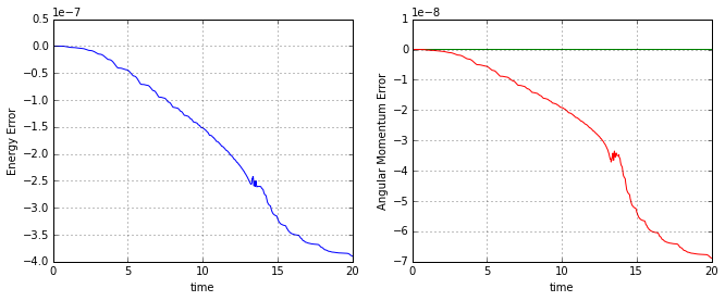
For comparison, the resulting conservation accuracy in the Coloumb case, shown below, is essentially the same.
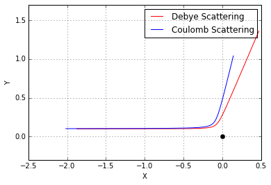
Based on the qualitative analysis of the potentials, we expect to see that Debye scattering gets closer to the scattering center and is deflected less than Coulomb scattering, all other things remaining the same. This is exactly what is observed.
With these initial validations done, the final step is to scan over a variety of impact parameters and then to compare the behavior of the scattering angle in the two cases. The same scan_impact_param function was used as in the last post with one modification. The calling sequence was modified to take an additional argument called model, which is a function pointer to the desired RHS of the equation of motion.
def scan_impact_param(b_range,s0,params,model):
    theta              = b_range[:]*0.0
    counter            = 0
    for b in b_range:
        timespan       = np.arange(0,20,0.001)
        s0[1]          = b
        soln           = ode(model,s0,timespan,args=(params,),rtol=1e-8,atol=1e-10)
        theta[counter] = scattering_angle(soln)
        counter        = counter + 1
    return theta
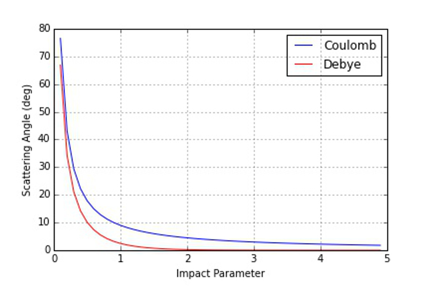
The resulting scattering plot shows, as expected, that the Debye potential allows the scattered particle closer access to the scattering center for a given scattering angle than does the Coulomb potential.
Next week, I’ll tidy up some odds and ends and close out this revisit of classical scattering.