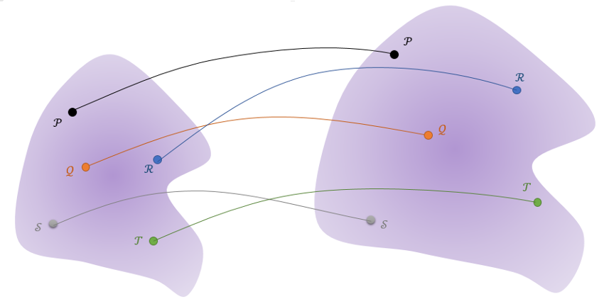
Last month’s post began a detailed study of continuum mechanics by looking at the general structure of the formalism and the specific linkage between the Lagrangian point-of-view, which co-moves along with a material element, and the Eulerian point-of-view, which focuses on specific locations and times as material elements move into and out of these locations.

The material derivative,

\[ \frac{d}{dt} f = \frac{\partial f}{\partial t} + \vec v \cdot \vec \nabla f \; , \]

provides the connection between these points-of-view, relating the time rate-of-change of the field $$f(t,\vec r)$$ as seen by the material element to the derivatives of the field at the instant that element passes through the position $$\vec r$$.

While the derivation of the material derivative given in the last post is mathematically correct, its abstract nature is difficult to internalize.  This post presents the material derivative in a variety of contexts to drive home the equivalence between the two points-of-view.

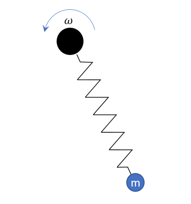
The physical model employed, consists of a material element, a small bit of fluid or elastic material (with enough internal cohesion that is stays as a discernable element), in motion around the Earth, which is, in turn, heated by the Sun.  The temperature that the element sees varies as it moves relative to the Earth-Sun line and with time as the Earth moves along its own orbit around the Sun, getting closer or further as the seasons change.

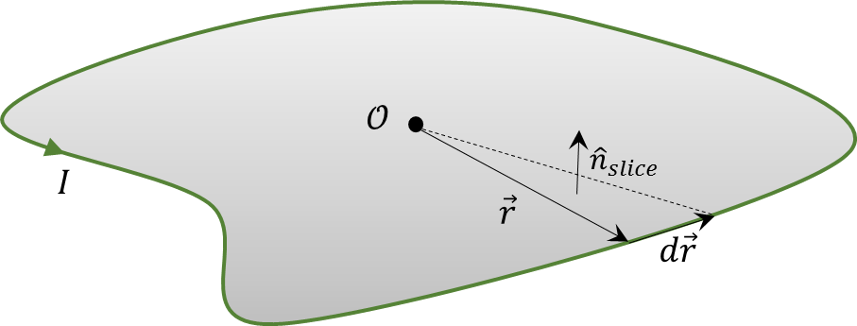
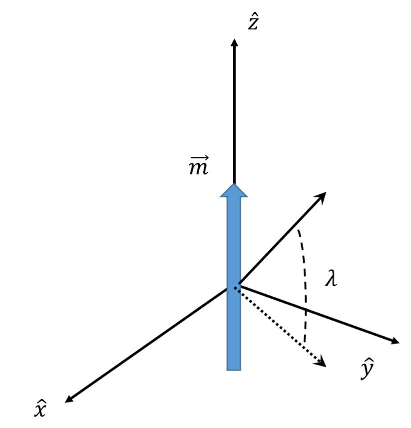
For simplicity, the geometry will be assumed 2-dimensional and will be, predominantly, described in plane polar coordinates $$r$$ and $$\theta$$.

The trajectory will be written as a product a radius function $$R(t) = R_0 + at$$ and a simple linear function for the polar angle $$\Theta = \omega t$$ associated with uniform circular motion ($$a$$ and $$\omega$$ are constants.  Depending on the context, the resulting trajectory may be expressed in either cartesian form as

\[ \vec R(t) = (R_0 + at) \left[ \cos(\omega t) \hat e_x + \sin (\omega t) \hat e_y \right] \;\]

and

\[ \vec V(t) = (R_0 + at) \left[ -\sin(\omega t) \hat e_x + \cos(\omega t) \hat e_y \right] \\ + at \left[ \cos(\omega t) \hat e_x + \sin(\omega t) \right] \hat e_y \; , \]

for the position and velocity, respectively, or

\[ \vec R(t) = (R_0 + at) \hat e_r(t) \; \]

and

\[ \vec V(t) = (R_0 + at) \hat e_{\theta}(t) + at \hat e_r(t) \; , \]

for the same in polar form.

Similarly, the temperature field will be written in separable form as a product of 3 functions, $$T_r$$, $$T_{\theta}$$, and $$T_t$$, which are functions solely of $$r$$, $$\theta$$, and $$t$$, respectively.  This last assumption, done for convenience, represents no loss of generality.  The specific form of each of these will be tailored to each of the three scenarios presented below.

In each scenario, the rate-of-change seen by the element (Lagrangian point-of-view) is calculated by the following process.  The position and velocity of the element is evaluated at tabulated times to produce an ephemeris, the temperature is measured at each of the ephemeris points, and then the time rate-of-change of the measured temperature is constructed by using the central difference approximation to the derivative given by

\[ \frac{d}{dt} T = \frac{T(t+\Delta t) – T(t-\Delta t)}{2 t} \; .\]

These values for the time rate-of-change define ‘truth’ in the Lagrangian point-of-view and will be the values against which we will judge the material derivative computation in the Eulerian point-of-view.

Scenario 1 – Time-independent Temperature Field Encountered in a Circular Orbit

In this scenario, the material element moves in a circular orbit ($$a=0$$) through the temperature field, defined by

\[ T(t,r,\theta) = T_0 (1 + \Delta T \cos(\theta) ) \exp\left(-r/r_0\right) \equiv T_{\theta} T_r \; .\]

This field is an elementary model of a hot Earth radiating its heat into space with a colder side (centered on $$\theta = \pi$$) pointing away from the Sun.

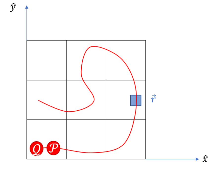
The element’s motion through the field (the colorbar maps the color to the temperature)

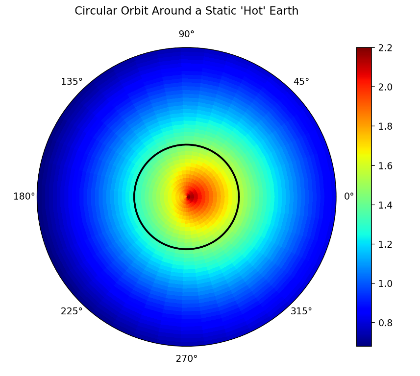
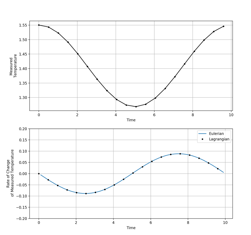
leads us to expect a periodic variation in time of the measured temperature, even though the underlying field is static (i.e. time-independent).

The gradient of the field, presented in the best way for numerical programming, is given by:

\[ \vec \nabla T = T_{\theta} T_{r,r} \hat e_r + \frac{1}{r} T_{\theta,\theta} T_r \hat e_{\theta} \; , \]

where:

\[ T_{r,r} \equiv \frac{\partial T_r}{\partial r} = -\frac{1}{r_0} \exp\left(-r/r_0\right) \; \]

and

\[ T_{\theta,\theta} \equiv \frac{\partial T_{\theta}}{\partial \theta} = -T_0 \Delta T \sin(\theta) \; .\]

The velocity in this scenario is entirely in the polar angle direction and is given by

\[ \vec V = R_0 \omega \hat e_{\theta} \; .\]

Since there is no explicit time dependence in the field, the right-hand or Eulerian side of the material derivative is

\[ \vec V \cdot \vec \nabla T = – R_0 \omega \frac{1}{R(t)} T_0 \Delta T \sin(\omega t) \exp\left( -R(t)/r0 \right) \; \, \]

where, it should be emphasized, the field gradients are evaluated at the instantaneous position of the material element.

Comparison of this expression to the Lagrangian truth from the central differences shows excellent agreement.

Scenario 2 – Time-independent Temperature Field Encountered in an Out-spiral Trajectory

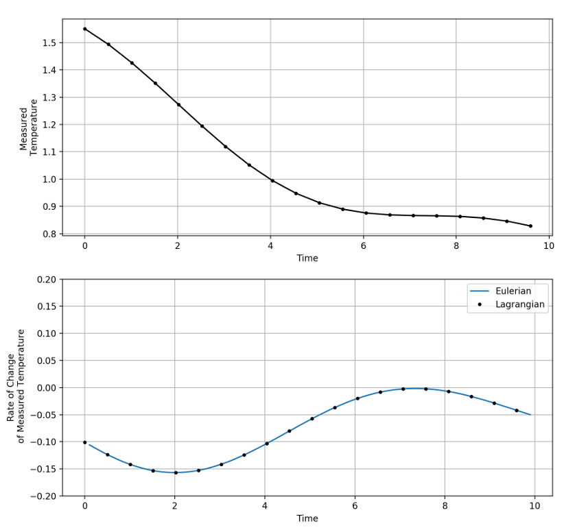
In this scenario, the underlying temperature field remains the same but the trajectory is an outgoing spiral ($$a>0$$)

and thus there are both radial and polar components of the velocity given by

\[ V_r = a t \]

and

\[ V_{\theta} = (R_0 + a t) \omega \; ,\]

respectively.

The Eulerian side of the material derivative now becomes

\[ \vec V \cdot \vec \nabla T = – a t \frac{1}{r_0} \exp\left(-r/r_0\right) T_0 (1 + \Delta T \cos(\omega t)) \\ – (R_0 + at) \omega \frac{1}{R(t)} T_0 \Delta T \sin(\omega t) \exp\left( -R(t)/r0 \right) \; . \]

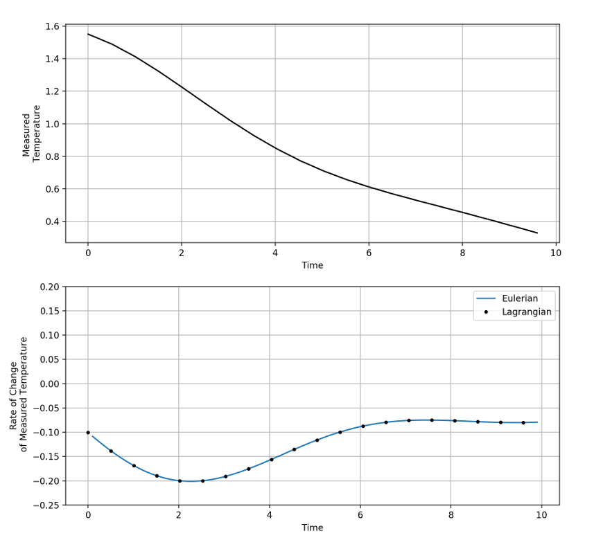
The measured temperature computed along the trajectory shows an overall, but not monotonic, decrease in the value, with the small bump upwards occurring when the material element swings to the hot side.  The time rate-of-change calculated in both ways again shows excellent agreement.

Scenario 3 – Time-dependent Temperature Field Encountered in an Out-spiral Trajectory

In this final scenario every possible variation is covered.  The trajectory is the same out-spiral used in Scenario 2.  To the spatial variation of the temperature field is added a simple time-dependence so that the temperature field is now:

\[ T(t,r,\theta) = T_r T_{\theta} exp(-t^2/\tau^2) \; .\]

The material derivative now includes a time variation of the field and the Eulerian form is

\[ \frac{\partial T}{\partial t} + \vec V \cdot \vec \nabla T = -\frac{2t}{\tau^2} T_t T_r T_{\theta} – a t \frac{1}{r_0} T_t T_r T_{\theta} \\ – (R_0 + at) \omega \frac{1}{R(t)} T_0 \Delta T \sin(\omega t) T_t T_r \; , \]

where $$T_r$$ and $$T_{\theta}$$ are evaluated at the ephemeris point of the material element $$\vec R(t)$$.

Once again, the agreement is excellent, demonstrating in a concrete fashion, the equivalence of Lagrangian and Eulerian points-of-view.

This post marks the beginning of a detailed study of continuum mechanics.  There are many reasons behind this study.  On the physical front, the applications are numerous and important.  Studies of elasticity are crucial in understanding the behavior of materials in diverse settings from man-made structures like cars, bridges, and buildings to naturally occurring applications like plate tectonics.  Fluid mechanics is ubiquitous, being involved in all aspects of industrial and academic endeavors.  Continuum mechanics also plays a role in such cutting-edge disciplines as plasma physics and general relativity.

Unfortunately, the study of continuum mechanics involves a number of difficulties at all levels of inquiry.

First and foremost is the philosophical difficulty associated with reconciling the atomic nature of matter with the concept of a continuous field.  Consider a portion of a substance whose atomic constituents are labeled

\[ \mathcal{P}, \mathcal{Q}, \mathcal{R}, \mathcal{S}, \mathcal{T} \; .\]

We imagine that each particle moves along a trajectory parameterized by $$t$$; that there is a mapping $$\Phi$$ that flows particle $$\mathcal{P}$$ from its position at $$\vec a_{\mathcal{P}}(t_0)$$  to $$\vec a_{\mathcal{P}}(t)$$:

\[ \Phi: \vec a_{\mathcal{P}}(t_0) \rightarrow \vec a_{\mathcal{P}}(t) \; . \]

Assuming the trajectories are continuous and smooth (i.e. putting aside the possibility of stochastic or quantum motion), so that the mapping $$\Phi$$ is differentiable, there remains many questions as to how a swarm of particles can be smeared or smoothed into a continuum.

The usual prescription is to employ the notion of a material or fluid element, whose volume is large enough to fit an enormous number of particles, so that smoothing can be done by taking averages, but small enough so that there are no appreciable changes across its extent.  That, this balancing act between the too small and the too large presents itself in many physical situations is one of the miracles of continuum mechanics.

There are additional considerations about any restrictions that should be placed on the continuum motion.  Can the trajectories cross so long as two elements don’t occupy the same point at the same time (see the above figure).  Do all the mathematical functions used in the model need to be single-valued, continuous, or differentiable?

The next set of difficulties involve a host of technical details.  Three stick out in particular: distinguishing between Lagrangian and Eulerian points-of-view, the mathematical way to construct the model of how the movement of the individual material particles will be tracked, and the eternal problem of notation and the associated bookkeeping.

In the Lagrangian viewpoint, attention is fixed on a material or fluid element and follows its motion as it flows.  This viewpoint is akin to sitting in a boat as it moves down a river.  The surroundings change and the banks slip by as the boat follows the piece of water on which it floats.  The Lagrangian viewpoint is the one in which Newton’s laws may be applied with almost the same ease as in particle mechanics.  The position, velocity, and acceleration of an element surrounding $$\mathcal{P}$$ follows the well-defined trajectory

\[ \vec a_{\mathcal{P}}(t) \; .\]

In the Eulerian viewpoint, attention is fixed on the locale and the various material or fluid elements which enter and leave this region are only briefly viewed before being lost.  Each airplane traveler who sits by the window over a wing and contemplates the lift generated as air rushes over it experiences the Eulerian viewpoint even if they are unaware of the finer points.  The Eulerian viewpoint is most commonly used in physical analysis since measurements are made at specific points and devices like valves and pipes and the like are fixed in space $$\vec r$$.

Connection between these two viewpoints is affected through the material derivative.

The material derivative, which has many aliases (such as the total or Lagrangian derivative – Wikipedia lists 10 of them), is based on the idea of how a set of trajectories fills a space.  Consider the path of two elements $$\mathcal{P}$$ and $$\mathcal{Q}$$ as they move along the red trajectory.

At some given time $$t_0$$ they are positioned as pictured at $$\vec a_{\mathcal{P}}$$ and $$\vec a_{\mathcal{Q}}$$.  At some later time $$t_1$$, $$\mathcal{P}$$ enters the blue box at $$\vec r$$.  Shortly afterwards, at $$t_2$$, $$\mathcal{Q}$$ enters the same position.  By noting the time and the starting point of each of these two elements, we can determine their respective positions at all later times.  Generalizing to a continuum, there exists, at least conceptually, a function

\[ \vec R(\vec a,t) \]

that spits out the position of an element that started at position $$\vec a$$ at time $$t_0$$.  A moment’s reflection should convince one that a proper boundary condition on $$\vec R$$ is

\[ \vec R(\vec a,t_0) = \vec a \; ,\]

that is the mapping is the identity at the initial time.

Since no two elements are allowed to occupy the same position at the same time, the function $$\vec R$$ can be inverted, again at least conceptually, so that we have a function

\[ \vec A(\vec r,t) \; .\]

This function works in a complementary fashion, telling us which of the elements is at $$\vec r$$ (blue box) at time $$t$$.  Its boundary condition at time $$t_0$$ has to be

\[ \vec A(\vec r,t_0) = \vec a \; , \]

since it has to coincide with $$\vec R$$ as an identity at the initial time ($$\vec A$$ and $$\vec R$$ are inverse mappings – if $$\vec R$$ is the identity then so must $$\vec A$$).

With this machinery in place, one can move back and forth between the trajectory (Lagrangian) and the field (Eulerian) points-of-view.

Now suppose that there are two observers, one that rides along with $$\mathcal{P}$$ and the other sitting in the blue box at $$\vec r$$, and suppose that each of them measures the temperature frequently.   Obviously, they must agree on the temperature only at $$t_1$$ when $$\vec R({\vec a_{\mathcal{P}},t_1}) = \vec r$$.  But will they agree on the rate of change in the temperature?

Generally, the answer is no for the following reason.   If the temperature field at each point and time in the space is given by $$T(x,y,z)$$ then the observer at $$\vec r$$ will see a rate of change of

\[ dT = \left. \frac{\partial T}{\partial t} \right|_{x,y=x_{\vec r},y_{\vec r}} dt \; ,\]

since the position remains unchanged (as emphasized by the standard notation on the partial derivative – for clarity of notation, this emphasis will be dropped hereafter).

The observer co-moving with $$\mathcal{P}$$ must plug his trajectory into $$T$$ to give

\[ T\left( X(\vec a,t), Y(\vec a,t), t \right) \]

with a corresponding change given by

\[ dT = \frac{\partial T}{\partial t} dt + \frac{\partial T}{\partial x} dx + \frac{\partial T}{\partial y} dy \; .\]

The time rate of change is given by dividing both sides by $$dt$$ to give

\[ \frac{dT}{dt} = \frac{\partial T}{\partial t} + \frac{\partial T}{\partial x} \frac{dx}{dt} + \frac{\partial T}{\partial y} \frac{dy}{dt} \; ,\]

which, in vector notation, gives the usual form of the material derivative

\[ \frac{dT}{dt} = \frac{\partial T}{\partial t} + \vec v \cdot \nabla T \; .\]

The next post will explore the material derivative in a concrete example. In the following posts, the material derivative will be the primary tool for relating Newton’s laws in the Lagrangian picture to the field equations in the Eulerian picture.

As pointed out in an article entitled Field Pattern of a magnetic dipole (Am. J. Phys. 68 (6), June 2000), J. P. Mc Tavish, notes that while it is common to see a treatment of the magnetic dipole in essentially every electromagnetic text, it is all too rare to find a discussion on how to draw the field lines. While Mc Tavish’s article is successful in remedying that shortfall, it omits any connection with specific physical situations, in particular with the most important dipole magnet to the human race: the one on which we live – the Earth.

Alternatively, in the space physics community it is all too common to see the physical connection to the Earth’s dipole field and corresponding field lines but the basic physics associated with deriving these equations from Maxwell’s equations to the dipole is usually missing. And those that do (e.g. the very instructive lecture by Ling-Hsaio Lyu) often cut some vital parts.

It is the intention of this post to create a single narrative that starts from first principles and ends with the standard space physics expression for the Earth’s dipole field in terms of the standard L-shells. The bulk of the initial part of this post is based on the treatment of the dipole in Foundations of Electromagnetic Theory by Reitz, Milford, and Christy.

The starting point is the monopole law $$\vec \nabla \cdot \vec B = 0$$, which asserts that the magnetic field is purely solenoidal, and, as a result, can be written in terms of the vector potential $$\vec A$$ as

\[ \vec B = \vec \nabla \times \vec A \; . \]

Since we want the description of an isolated magnetic dipole field, two immediate conditions can be place on Maxwell’s equations: $$\partial_t \vec B = 0$$ and $$\rho = 0$$. The only non-trivial Maxwell equation is now the Ampere-Maxwell law, that states (subject to the earlier conditions)

\[ \vec \nabla \times \vec B = \mu_0 \vec J \; . \]

Substituting in the vector potential yields

\[ \vec \nabla \times (\vec \nabla \vec A) = \mu_0 \vec J \; .\]

Expanding the double-curl with the standard vector identity leads to

\[ \vec \nabla (\vec \nabla \cdot \vec A) – \nabla^2 \vec A = \mu_0 \vec J \; , \]

which can be further reduced by picking the Lorentz gauge, which sets $$ \vec \nabla \cdot \vec A = 0 $$. This choice leads to the final equation

\[ \nabla^2 \vec A = -\mu_0 \vec J \; ,\]

which asserts that each component of the vector potential obeys a Poisson equation with the source being $$\mu_0 \vec J$$. The solution of these three equations follows by analogy with electrostatics and the result is

\[ \vec A(\vec r) = \frac{\mu_0}{4 \pi} \int d^3 r’ \frac{\vec J(\vec r \,’)}{|\vec r – \vec r \,’|} \; . \]

Now for most dipoles (microscopically contained in matter or the Earth), the field is generally distant from the source point ($$|\vec r| >> |\vec r \,’| $$). This relation suggests a multipole expansion of the Green’s function

\[ |\vec r – \vec r \,’|^{-1} = (r^2 + r’^2 – 2 \vec r \cdot \vec r \,’)^{-1/2} \; . \]

The dipole is the first-order piece of such an expansion, so we can approximate the Green’s function as

\[ |\vec r – \vec r \,’|^{-1} = \frac{1}{r} \left[ 1 + \frac{\vec r \cdot \vec r \,’}{r^2} \right] \; . \]

One additional approximation is needed; assume that the currents creating the dipole are bound and an be idealized as flowing through a “thin wire” (effectively a Dirac delta function is used to localize the current into a circuit whose characteristic sizes are small compared to all other lengths being considered). In this case, the volume integral becomes a closed line integral. Under this modest approximation:

\[ \vec A(\vec r) = \frac{\mu_0 I}{4 \pi} \left\{ \frac{1}{r} \oint d \vec r \,’ + \frac{1}{r^3} \oint d \vec r \,’ \vec r \cdot \vec r \,’ \right \} \; . \]

The first integral vanishes since the line integral forms a close loop. The second integral, refered hereafter as the dipole integral, requires some ingenuity, all of which is supplied by Rietz, Milford, and Christy (Sec. 8.7). The first step in dealing with the dipole integral comes from noting (using back-cab) that

\[ (\vec r \,’ \times d \vec r \,’) \times \vec r = – \vec r \times (\vec r \,’ \times d \vec r \,’) = \\ – [ \vec r \,’ (\vec r \cdot d \vec r \,’) – d \vec r \,’ (\vec r \cdot \vec r \,’) ] = d\vec r \,’ (\vec r \cdot \vec r \,’) – \vec r \,’ (\vec r \cdot d \vec r \,’) \; .\]

To eliminate the first term employ the identity

\[ d[ \vec r \,’ (\vec r \cdot \vec r \,’) ] = d \vec r \,’ (\vec r \cdot \vec r \,’) + \vec r \,’ (\vec r \cdot d \vec r \,’) \; \]

that results from a change in $$\vec r \,’$$ keeping $$\vec r$$ fixed.

Now add the two previous expressions together to get

\[ (\vec r \,’ \times d \vec r \,’) \times \vec r + d[ \vec r \,’ (\vec r \,’ \cdot \vec r) ] = 2 d \vec r \,’ (\vec r \cdot \vec r \,’) \; , \]

which, when divided by 2 and substituted into the dipole integral gives

\[ \vec A (\vec r) = \frac{\mu_0 I}{4 \pi r^3} \frac{1}{2} \oint \left\{ (\vec r \,’ \times d \vec r \,’) \times \vec r + d[\vec r \,’ (\vec r \,’ \cdot \vec r) ] \right \} \; . \]

The second terms is identically zero, since it an exact differential. The first terms can be suggestively rearranged to give

\[ \vec A(\vec r) = \frac{\mu_0}{4 \pi} \left\{ \oint \frac{I}{2} (\vec r \,’ \times d \vec r \,’) \right\} \times \frac{\vec r}{r^3} \equiv \frac{\mu_0}{4 \pi} \vec m \times \frac{\vec r}{r^3} \; , \]

where $$\vec m$$ is defined as the magnetic dipole (or magnetic dipole moment).

Before computing $$\vec B$$, let’s take a moment to think about the definition of $$\vec m$$. Consider an arbitrary current-carrying loop

where the origin is chosen near the loop. The differential vector $$\vec r \,’ \times d \vec r \,’$$ is normal to a small slice of area. Summing each piece in the integral results in an expression that roughly says

\[ \vec m = \frac{\mu_0}{4 \pi} I \left( \frac{1}{2} \oint \vec r \,’ \times d \vec r \,’ \right) = \frac{\mu_0}{4 \pi} I \, Area \, \hat n \; , \]

but the area has each slice weighted differently, based on how far from the origin it excursion takes it. As a side note, Griffiths calls this the directed area and obtains it from the Stoke’s theorem by an ingenious substitution for the vector field in question (seems like some degree of cleverness is required no matter how one does this analysis).

The next step is to calculate the magnetic field. Taking the curl gives

\[ \vec B (\vec r) = \vec \nabla \times \vec A(\vec r) = \vec \nabla \times \left( \frac{\mu_0}{4 \pi} \vec m \times \frac{\vec r}{r^3} \right) \; .\]

To expand the right-hand side, use index notation (starting with $$\vec A \times \vec B = \epsilon_{ijk} A_j B_k$$)

\[ \vec \nabla \times \left( \frac{\mu_0}{4 \pi} \vec m \times \frac{\vec r}{r^3} \right) = \frac{\mu_0}{4 \pi} \epsilon_{ijk} \epsilon_{k \ell m} \partial_j m_{\ell} \frac{r_m}{r^3} \; . \]

Cyclically permute the indices on $$\epsilon_{k \ell m}$$ to get

\[ \frac{\mu_0}{4 \pi} \epsilon_{ijk} \epsilon_{k \ell m} \partial_j m_{\ell} \frac{r_m}{r^3} = \frac{\mu_0}{4 \pi} \epsilon_{ijk} \epsilon_{\ell m k} \partial_j m_{\ell} \frac{r_m}{r^3} \; . \]

Now use the standard identity

\[ \epsilon_{ijk} \epsilon_{\ell mk} = \delta_{i \ell} \delta _{jm} – \delta_{im} \delta_{j \ell} \; .\]

to get

\[ \frac{\mu_0}{4 \pi} \epsilon_{ijk} \epsilon_{\ell m k} \partial_j m_{\ell} \frac{r_m}{r^3} = \frac{\mu_0}{4 \pi} \left( \delta_{i \ell} \delta _{jm} – \delta_{im} \delta_{j \ell} \right) \partial_j m_{\ell} \frac{r_m}{r^3} \; .\]

Expanding gives

\[ \frac{\mu_0}{4 \pi} \epsilon_{ijk} \epsilon_{\ell m k} \partial_j m_{\ell} \frac{r_m}{r^3} = \frac{\mu_0}{4 \pi} \left[ m_i \partial_j \left( \frac{r_j}{r^3} \right) – m_j \partial_j \left( \frac{r_i}{r^3} \right) \right ] \; .\]

Now focus on the term inside the square brackets. Operating with the derivatives gives

\[ m_i \partial_j \left( \frac{r_j}{r^3} \right) – m_j \partial_j \left( \frac{r_i}{r^3} \right) = m_i \frac{3}{r^3} – 3 m_i \frac{r_j r_j}{r^5} – m_j \frac{\delta_{ij}}{r^3} + m_j \frac{3 r_i r_j}{r^5} \; . \]

The first two terms vanish and the second two, when put into vector notation, give for the magnetic field

\[ \vec B(\vec r) = \frac{\mu_0}{4 \pi} \left[ -\frac{\vec m}{r^3} + 3 \frac{(\vec m \cdot \vec r) \vec r}{r^5} \right] \; .\]

With this form in hand, it is possible to calculate the field lines. There are two ways to do this: in Cartesian coordinates and in spherical coordinates. Either is fine, but spherical coordinates affords some advantages in space physics and will be pursued here.

That said, both cases benefit from exploiting axial symmetry and, without loss of generality, the analysis will be confined to the $$x-z$$ plane.

The geometry is shown below.

To put the coordinate-free expression into polar coordinates we need to express the vectors in terms of the basis $$\left\{ \hat r, \hat \lambda, \hat \phi \right\}$$ (although we are supressing $$\hat \phi$$ by exploiting the azimuthal symmetry).

Starting with the position vector

\[ \vec r = r \cos \lambda \, \hat x + r \sin \lambda \, \hat z \; \]

gives

\[ \hat r = \frac{\partial \vec r}{\partial r} = \cos \lambda \, \hat x + \sin \lambda \, \hat z \; , \]

and

\[ \hat \lambda = \frac{\partial \vec r}{\partial \lambda} / \left| \frac{\partial \vec r}{\partial \lambda} \right| = – \sin \lambda \, \hat x + \cos \lambda \, \hat z \; . \]

Inverting these relations gives

\[ \hat z = \sin \lambda \, \hat r + \cos \lambda \, \hat \lambda \; .\]

Since $$\vec m = m \hat z$$, the magnetic field becomes

\[ \vec B = \frac{m \mu_0}{4 \pi r^3} \left[ 3 \frac{ (\vec m \cdot \vec r) \vec r }{r^2} – \vec m \right] = \frac{m \mu_0}{4 \pi r^3} \left[ 2 \sin \lambda \, \hat r – \cos \lambda \, \hat \lambda \right] \; , \]

giving

\[ B_r = \frac{D}{r^3} 2 \sin \lambda \; \]

and

\[ B_{\lambda} = \, -\frac{D}{r^3} \cos \lambda \; , \]

where $$D = m \mu_0 /4 \pi$$.

The final piece is to get an equation of the form $$r = r(\lambda)$$ so that we can get the field lines. From Section 3.2 of Introduction to Vector Analysis by David and Snider, the tangent field to the field lines is given by $$\vec T = \beta \vec B$$, where $$\beta$$ is an arbitrary, and ultimately, inconsequential, constant. In coordinates, this expression leads to the vector equation

\[ \vec T = \frac{d r}{d s} \hat r + r \frac{d \lambda}{d s} \hat \lambda = B_r \hat r + B_{\lambda} \hat \lambda \; , \]

which gives

\[ \frac{dr}{B_r} = \frac{r d \lambda}{B_{\lambda}} \; . \]

This equation is recast as follows:

\[ \frac{dr}{r} = \frac{B_r}{B_{\lambda}} d \lambda = \, – \frac{2 \sin \lambda}{\cos \lambda} d \lambda = 2 \frac{d(\cos \lambda)}{\cos \lambda} \; . \]

The solution is readily obtained by integrating from the equation towards the pole (symmetry again)

\[ \int_{r_{eq}}^{r} \frac{dr’}{r’} = \int_{1}^{\cos \lambda} 2 \frac{ d(\cos \lambda) }{ \cos \lambda } = \int_{1}^{\cos \lambda} 2 \frac{ dx }{x} \; , \]

giving

\[ \left. \ln(r’) \right|^r_{r_{eq}} = \left. \ln( x^2 ) \right|_1^{\cos \lambda} \; , \]

which simplifies to

\[ \ln(r)- \ln(r_{eq}) = \ln(\cos^2 \lambda) – \ln(1) \; . \]

The final form is

\[ r(\lambda) = r_{eq} \cos^2 \lambda = L R_e \cos^2 \lambda \; . \]

The parameter $$L$$ labels the fieldline and different fieldlines intersect the Earth’s surface at different latitudes.

`

As part of the special New Years list theme issue, this month’s column is going to propose a ranking for the top 10 Nobel Prizes in physics out of the 117 that have been awarded.  The primary criterion employed is that the work had to have a profound effect on the daily human quality of life in contrast to having a deep and lasting influence on our general knowledge of the universe.  The recent buzz about the discovery of the Higgs boson captured the imaginations of the public at large and advanced our knowledge of the fundamental laws of nature but has currently had no practical impact on the day-to-day lives of most people.  The energies required to unleash the Higgs are enormous and the idea that Higgs physics will be featured in the latest tech gadget absurd.  Thus, its discovery has no place on this list, even though it was an amazing accomplishment.

Each entry in the list will be cited first with the year, followed by the text the Nobel committee used to describe the discovery followed by the person or persons to whom the prize was awarded.  For those prizes where more than one discovery was recognized, the ordering will be alphabetical.

10.       1918:  Discovery of elemental quanta – Max Planck

The one that started the whole enterprise of quantum mechanics.  When faced with the puzzle of how to solve the ultraviolet catastrophe in the modeling of black body radiation, Planck proposed a radical concept:  the energy in an oscillating mode couldn’t be any arbitrary value but had to be a multiple of some elementary packet of energy.  The fact that is fit the experimental data so well launched a mode of physical investigation that enabled all of the incredible technology that we all enjoy.

9.         1989:  Development of Methods to Isolate Atoms and Subatomic Particles for study; Development of the Atomic Clock – Hans Georg Dehmelt, Wolfgang Paul, Norman Foster Ramsey

This entry is primarily on the list due to the last cited development of the atomic clock.  It is hard to reckon how important good time keeping and synchronization is to the underlying aspects of human activity.  Knowing when to plant is vital to good harvests; knowing when to debit or credit an account is vital to good business; and knowing how to accurately keep good time opens the door for greater exploration of the universe.

8.         2007: Discovery of Giant Magnetoresistance – Albert Fert and Peter Grunberg

The digital age has profoundly enriched lives all over the world and this entry is the first of 3 concerning that aspect of our lives.  The discovery of giant magnetoresistance immensely increased the areal density of information that could be stored on hard drives and it is the most important reason why huge amount of data can be placed in clouds and servers.  Each of us is now endowed with the ability to store and access digital data in a way that only the richest corporations could a few decades earlier.  It is not an over-statement to conclude that the new fields of data science and machine learning would not be possible with this discovery.

7.         1929: Discovery of the Wave Nature of Electrons – Louis-Victor de Broglie

What Planck began with his quantization of radiation, de Broglie finished with his proposal that matter had a wave-like nature of its very own.  Arguing from symmetry and well-established physical models of classical mechanics, de Broglie’s idea of matter waves solidified quantum mechanics as the preeminent science and paved to way for the formal development of the theory by Heisenberg, Schrodinger, Born, and Dirac.

6.         1952:  Discovery of Nuclear Magnetic Resonance in Solids – Felix Bloch and E.M. Purcell

Nuclear magnetic resonance is one of the two non-destructive imaging techniques on this list.  Mostly known under its more politically-correct name of magnetic resonance imaging, this technique complements the use of X-rays in viewing the inner workings of the body with invasive surgery.  It also has applications beyond medical imaging in a variety of situations where non-destructive investigation is required.

5.         1945:  Discovery of the Exclusion Principle of Electrons – Wolfgang Pauli

Like the discoveries of Planck and de Broglie, Pauli’s idea is profound not for it intrinsic nature but for the doors it opened.  Advances in chemistry and material sciences, research fields that have opened up miracle drugs and novel new plastics, semi-conductors, and other materials would not have happened without the idea that electrons pack into an atom in a way that prevents them from having the same quantum numbers.

4.         2009:  Achievements Concerning the Transmission of Light in Fibres for Optical Communication;  Invention of the CCD Sensor, an Imaging Semiconductor Circuit – Willard Boyd and George Smith; Charles Kao

We all take for granted the ability to take out a phone to film or photograph something of interest to us and to use the information superstructure to post or share what we’ve captured with others.  In this way we communicate with love ones not present and memorialize for later study.  In this way, we also make up an army of citizen-journalists who have created a new type of politics not filtered through official channels.   All of this is having a profound effect on society and is enabled by the CCD and the fiber optics.  I’ve often thought that perhaps the best name for this entry is the YouTube prize.

3.         1901:  Discovery of X-Rays – Wilhelm Conrad Rontgen

The first Nobel Prize ever awarded, Rontgen’s discovery of X-Rays was also the first type of non-invasive imaging.  Due to their ability to penetrate matter, X-Rays allowed the first views into the workings of the human body without the need to cut it open.  Broken bones, infections, and tumors are only some of the maladies that could be treated with greater precision and with less pain for the patient.  X-Rays also proved useful in investigating the goodness of welds, the stability of structures, and the like.

2.         1956: Investigations on Semiconductors and Invention of the Transistor – John Bardeen, Walter H. Brattain, William B. Shockey

It is hard to underestimate the importance of the transistor.  Without it, logical gates, programming and practical computing, the entire digital age would not have come about.  The idea that millions of these devices can be packed into an area about the size of a postage stamp staggers the imagination.  And, as we are just at the beginning the road, it is hard to see just where all of this technology will lead.  But one thing is certain, the transistor has had one of the most profound influences on society of any modern human invention.

1.         1909: Development of Wireless Telegraphy – Ferdinand Braun and Guglielmo Marconi

And number one on the list is Braun’s and Marconi’s invention of radio.  ‘Wireless Telegraphy’, as the Nobel Committee called it, ushered in telecommunications and all that comes in its train: television, cell phones, radio, wireless routers, etc..  Man is a social creature and language is the glue that holds society together.  Telecommunications allows the reach of language to go further linking far-away with close-to-home.  No other entry in this list has done more to knit the world together as a single family.

In the last two posts, the role of constraints in a mechanical system and the methods for incorporating them have been explored. Among the things that were demonstrated were the facts that the Newton approach was ill-suited to the inclusion of constraints while the Lagrangian method is better equipped, and that within the Lagrangian method there are two approaches for incorporating the constraints: 1) direct elimination in the event the constraints are holonomic, and 2) the use of the Lagrange multipliers. The earlier analysis of the pendulum showed how to analytically use the Lagrange multipliers and demonstrated, in detail, that the multiplier was the force of constraint.

This post returns to the problem of a bead moving down a wire and shows that, whereas the Newtonian approach fails, the Lagrangian approach works nicely. The starting point is the Lagrangian

\[ L = \frac{1}{2} m (\dot x^2 + \dot y^2 ) – m g y + \lambda ( y – f(x) ) \; ,\]

with both $$x$$ and $$y$$ as dynamical degrees of freedom augmented with a Lagrange multiplier that enforces the constraint equation $$y= f(x)$$.

The conjugate momenta are

\[ p_x = \frac{\partial L}{\partial \dot x} = m \dot x \; \]

and

\[ p_y = \frac{\partial L}{\partial \dot y} = m \dot y \; . \]

The corresponding generalized forces are

\[ Q_x = \frac{\partial L}{\partial x} = – \lambda f’ \; ,\]

where $$f’$$ is the derivative of the constraint function $$f(x)$$ with respect to $$x$$, and

\[ Q_y = \frac{\partial L}{\partial \dot y} = – m g + \lambda \; ,\]

The equations of motion are

\[ \ddot x = -\frac{\lambda}{m} f’ \; \]

and

\[ \ddot y = -g + \frac{\lambda}{m} \; .\]

Since the ratio of the Lagrange multiplier to particle mass appears in each equation (i.e., the constraint force per unit mass), it is natural and convenient to define $$\lambda_m = \frac{\lambda}{m}$$ and to work with that quantity going forward.

Since the $$y$$ degree of freedom is related to $$x$$ through the constraint, there is a kinematic relationship that requires

\[ \dot y = \frac{d}{dt} f(x) = \frac{d f}{d x} \frac{dx}{dt} = f’ \dot x \]

and

\[ \ddot y = \frac{d}{dt} \dot y = \frac{d}{dt}( f’ \dot x ) = f” \dot x^2 + f’ \ddot x \; .\]

To determine the Lagrange multiplier, equate the dynamic expression for $$\ddot y$$ with the kinematic one to get

\[ -g + \lambda_m = f” \dot x^2 + f’ \ddot x \; .\]

The next step eliminates the $$x$$ acceleration by substituting-in its equation of motion giving

\[ -g + \lambda_m = f” \dot x^2 – f’^2 \lambda_m \; , \]

which can be easily solved for

\[ \lambda_m = \frac{ f” \dot x^2 + g}{1 + f’^2} \; . \]

This expression of the constraint force per unit mass is similar to the expressions in the earlier analysis but differs in one key way with the inclusion of the velocity-dependent piece proportional to $$\dot x^2$$. This constraint acceleration is now equipped to generate additional force (not just the expected normal force on the surface) as numerical errors move the motion off of the constraint. Of course, this is not a miraculous result and the constraint had been used to link the $$x$$ and $$y$$ equation of motion, but it is cleaner than the earlier method, it provides the constraint force, and, most important, it provides a mechanism for calculating the kinematics in a more convenient way than the solve-for-$$x$$-and-then-deduce method of that earlier post. As a reminder, those state-space equations were

\[ \frac{d}{dt} \left[ \begin{array}{c} x \\ y\\ \dot x \\ \dot y \end{array} \right] = \left[ \begin{array}{c} \dot x \\ \dot y \\ – g \tau f’ \\ – g \tau f’^2 \end{array} \right] \; ,\]

where $$\tau = (1+f’^2)^{-1}$$.

The Lagrange multipliers form of the equations of motion are also easy to code and couple to a standard solver. As in the earlier post, I used the Python and SciPy ecosystem with the primary function being:

def roller_coaster_multipliers(state,t,geometry,g):
    #unpack the state
    x  = state[0]
    y  = state[1]
    vx = state[2]
    vy = state[3]
    
    #evaluate the geometry
    f,df,df2 = geometry(x)
    
    #calculate the lagrange multiplier per unit mass
    lam_m = ( df2*vx*vx + g )/(1.0 + df*df)
   
    return np.array([vx,vy,-lam_m*df,lam_m - g])

where the function geometry can be any curve in the $$x-y$$ plane. For example, for a bead sliding down a parabolic-shaped wire $$y = x^2$$, the corresponding function is

def parabola(x):
    return x**2, 2*x, 2

and the assignment

  geometry = parabola

provides this shape to the solver.

The results for the motion are

showing excellent agreement with the constraint for over two oscillations and good agreement with energy conservation.

This approach offers a nice alternative to the earlier 1-D approach in that all the dynamical degrees of freedom are present and, as a result, the kinematics are cleaner. In addition, the actual constraint force, taking into account deviations away from the surface, is computed. This is an important feature and one that can’t be obtained otherwise, since we can only compute the normal force at the surface and not away from it on either side.

In the spirit of simplicity embraced by the last post, this month’s analysis also deals with motion in one-dimension. As shown in that analysis, the naive application of Newton’s laws to motion of a bead along a curved wire failed except in the simplest of cases – that of motion along a straight line (i.e., essentially down an inclined plane). Instead, Lagrange’s method was used where one of the dynamical degrees of freedom was eliminated by direct substitution of the constraint into the Lagrangian. This post examines another (deceptively) simple problem, the motion of a bob at the end of an ideal pendulum, and compares and contrasts direct substitution of the constraint with the use of Lagrange multipliers. The idea is to examine how Lagrange multipliers work and what information they provide in a problem where one can easily understand all the ‘moving parts’. The content of the post is inspired by the fine write-up on Lagrange multipliers by Ted Jacobson for a course on classical mechanics. I’ve taken Jacobson’s basic discussion on Lagrange multipliers and extended it in several directions; nonetheless, the insights on that particular topic are due to him.

To begin, assume that the pendulum bob can move in the plane subject to the forces of gravity and of an inextensible rod of length $$R$$ to which the bob is attached.

The Lagrangian for arbitrary two-dimensional motion, subjected to gravity along the $$x$$-direction, expressed in plane polar coordinates is

\[ L = \frac{1}{2} m \left( \dot \rho^2 + \rho^2 \dot \phi^2 \right) + m g r \cos \phi \; , \]

where the zero of the potential energy is taken to be the lowest point in the bob’s motion and where the constraint $$\rho = R$$ has not yet been used.

Before digging into the Lagrangian method, it is worth taking a step back to see how this system is described in the Newtonian picture. The forces on the bob at any given point of the motion in the plane lead to a vector equation that is determined by the well-known form of the acceleration in terms of the radial and azimutal unit vectors

\[ \ddot {\vec r} = (\ddot \rho – \rho \dot \phi^2) \hat e_{\rho} + (2 \dot \rho \dot \phi + \rho \ddot \phi) \hat e_{\phi} \; . \]

Applying Newton’s laws to the force vectors shown in the figure gives

\[ m g \cos \phi – T = m (\ddot \rho – \rho \dot \phi^2 ) \; \]

and

\[ -m g \sin \phi = m ( 2 \dot \rho \dot \phi + \rho \ddot \phi )\; .\]

Because the radius is fixed at $$\rho = R$$, the kinematics of the pendulum require $$\dot \rho = 0$$ and $$\ddot \rho = 0$$. The first equation provides a mechanism for calculating $$T$$ as

\[ T = m g \cos \phi + m R \dot \phi^2 \; .\]

The second equation gives the classic equation of motion for the pendulum

\[ R \ddot \phi + g \sin \phi = 0 \; .\]

These simple equations will help in interpretting the Lagrangian analysis.

Directly Impose the Constraint

Since the constraint is holonomic, it can be directly imposed on the Lagrangian, allowing for the radial degree of freedom to be eliminated, yielding

\[ L = \frac{1}{2} m R^2 \dot \phi^2 + m g R \cos \phi \; . \]

The conjugate momentum is

\[ p_{\phi} = m R^2 \dot \phi \; , \]

the generalized force is

\[ Q_{\phi} = – m g R \sin \phi \; , \]

and the resulting equation of motion is

\[ R \ddot \phi + g \sin \phi = 0 \; , \]

exactly the result obtained from Newton’s laws, where computation of $$\hat e_{\rho}$$ and $$\hat e_{\phi}$$ and slogging through a vector set of equations was needed.

It is worth noting how much easier it was to get to these equations than the path through Newton’s laws.

Using Lagrange Multipliers

The alternative way of handling the constraint is by leaving both degrees of freedom (radial and azimuthal) in the Lagrangian, augmenting it with the dynamical constraint. The key is in determining how this augmentation is to be done.

Jacobson argues from analogy with multi-variable calculus. In order to optimize a function $$f(x,y,z)$$ subject to a constraint $$C(x,y,z) = 0$$, one must limit the gradient of the function so that

\[ df = – \lambda d C \; . \]

Since $$C=0$$,

\[ \lambda d C = C d\lambda + \lambda d C = d( \lambda C) \; . \]

This manipulation allows for the combination $$d(f + \lambda C)$$ to now represent an unconstrained optimization problem. In the event there are multiple constraints, each constraint gets a corresponding Lagrange multiplier and is added to the function.

The generalization to variational problems comes by identifying $$f$$ as the action $$S$$. The interesting part is the generalization required to include the constraints. Since the constraint is active at each point of the motion, there are an infinity of constraints, and each one must be included in the action at each time by integration. The resulting unconstrained variational principle is

\[ \int dt (L + \lambda(t) C(t)) \; .\]

The new Lagrangian is

\[ L’ = L + \lambda C = \frac{1}{2} m (\dot \rho^2 + \rho^2 \dot \phi^2) + m g \rho \cos \phi + \lambda (\rho – R) \; . \]

The corresponding radial equation is

\[ m \ddot \rho = m \rho \dot \phi^2 + m g \cos \phi + \lambda \; \]

and the azimuthal equation

\[ m \rho^2 \ddot \phi + 2 m \rho \dot \rho \dot \phi + m g \rho \sin \phi = 0 \; . \]

To these equations must be added the constaint to yield

\[ \lambda = – m \rho \dot \phi^2 – m g \cos \phi \; . \]

and

\[ m R^2 \ddot \phi + m g R \sin \phi = 0 \; . \]

Thus we can identify $$\lambda = T$$, the force of constraint.

This is a general feature of the Lagrange multipliers. They incorporate the constraint into the variation and we are free to ignore it if we want only the dynamics, or we can use $$\lambda$$ to determine if it is explicitly desired.

This post begins a multi-part exploration of the role of constraints in mechanical systems. It builds on the general framework discussed in the last post but does so by examining specific examples. This month the focus will be on the simplest example of a constraint: a bead sliding on a wire.

Despite its trivial appearance, this problem is surprisingly complex due to the presence of the constraint and, as will be shown below, provides significant obstacles to obtaining an accurate numerical solution.

The following figure shows a portion of the wire, the position, $$\vec r$$, and the velocity, $$\vec v$$, of the bead, and the two forces acting upon it; namely the force of gravity $${\vec F}_g$$ and the normal force $${\vec F}_N$$. With this information, it is, in principle, easy to solve for the motion of the bead via Newton’s laws. There are several equivalent ways of carrying this out but I’ll be focusing on the most geometric of these.

The position of a particle in a plane is given by

\[ \vec r = \left[ \begin{array}{c} x \\ y \end{array} \right] \; . \]

Since the bead must remain on the wire, only those values of $$y$$ satisfying $$y = f(x)$$ are permissible and the position can now be written as

\[ \vec r = \left[ \begin{array}{c} x \\ f(x) \end{array} \right ] \; . \]

The velocity is then given by

\[ \vec v = \left[ \begin{array}{c} 1 \\ f'(x) \end{array} \right] \dot x \; .\]

The normal to the curve, $$\hat N$$, is obtained from the requirement that motion consistent with the constraint must always be perpendicular to the normal to the wire at the point in question:

\[ \hat N \cdot d\vec r = N_x dx + N_y dy = 0 \;.\]

Using the constraint equation $$y – f(x) = 0$$ and then taking the differential yields the component form

\[ dy – f'(x) dx = 0 \; , \]

from which it is easy to read off the components of the normal (the sign being chosen so that $$\vec F_N$$ is in opposition $$\vec F_g$$. Subsequent normalization gives

\[ \hat N = \frac{1}{\sqrt{1+f’^2}} \left[ \begin{array}{c} -f'(x) \\ 1 \end{array} \right] \; .\]

The forces on the bead are due to gravity

\[ \vec F_g = – m g \hat y \]

and the normal force

\[ \vec F_N = -(\vec F_g \cdot \hat N) \hat N = \frac{m g}{1+f’^2} \left[ \begin{array}{c} -f’ \\ 1 \end{array} \right]\; \]

For notational convenience in what follows, define

\[ \tau = \frac{1}{1+f’2} \; .\]

Summing the forces and inserting them into Newton’s second law leads to the following equations (eliminating $$m$$ from both sides)

\[ \left[ \begin{array}{c} \ddot x \\ \ddot y \end{array} \right] = \left[ \begin{array}{c} -g \tau f’ \\ g (\tau -1 ) \end{array} \right] = \left[ \begin{array}{c} -g \tau f’ \\ – g \tau f’^2 \end{array} \right] \; .\]

Expressing Newton’s equations in state-space form then yields

\[ \frac{d}{dt} \left[ \begin{array}{c} x \\ y\\ \dot x \\ \dot y \end{array} \right] = \left[ \begin{array}{c} \dot x \\ \dot y \\ – g \tau f’ \\ – g \tau f’^2 \end{array} \right] \; .\]

These equations are easy to code and couple to a standard solver. I chose to implement this system in Python and SciPy as follows:

def roller_coaster(state,t,geometry,g):
    #unpack the state
    x     = state[0]
    y     = state[1]
    vx    = state[2]
    vy    = state[3]
    
    #evaluate the geometry
    f,df,df2 = geometry(x)
    tau      = 1.0/(1.0+df**2)
    
    #return the derivative
    return np.array([vx,vy,-g*tau*df,-g*tau*df**2])

where the function geometry can be any curve in the $$x-y$$ plane. For example, for a bead sliding down a parabolic-shaped wire $$y = x^2$$, the corresponding function is

def parabola(x):
    return x**2, 2*x, 2

and the assignment

  geometry = parabola

provides this shape to the solver.

The first case studied with this formalism was where the wire shape is a simple straight segment, parallel to the edge of an inclided plane and refered to as such for the sake simplicity. The resulting motion was consistent with the shape

and the energy

was very well conserved.

These good results failed to hold when the shape of the wire was made parabolic. The resulting motion stayed on the parabola for a short time but eventually departed from the constraint by dropping below

while simultaneously showing a large deviation

from the initial energy.

The situation was no different for other geometeries tried. The problem seems to lie in the fact that the normal force is unable to respond to numerical errors. As the constraint begins to be violated, the wire is unable to conjure additional force to enforce it. The Newton method, while attractive from its simplicity, is simply inadequate for working with all but the most trivial of constraints.

The usual way of addressing this problem is to eliminate one degree of dynamical freedom. Either $$x$$ or $$y$$ has to go and the conventional approaches seem to favor $$x$$ as the parameter that stays. Again, there are several ways to effect this change but in this case both are worth examining.

In the first method, Newton’s equations are used to eliminate the $$y$$ in favor of $$x$$ by combining their equations of motion by first expressing

\[ -\frac{\ddot x}{g f’} = \tau \]

and then by inserting the left-hand side into the $$y$$ equation yielding

\[ \ddot y + g = -\frac{\ddot x}{f’} \; .\]

Solving this to give

\[ \ddot x = -f'(\ddot y + g) \]

and then using

\[ \dot y = \frac{df}{dx} \dot x = f’ \dot x \]

and

\[ \ddot y = f’ \ddot x + f” \dot x^2 \; . \]

The final equation, after substitution for $$\ddot y$$ has been made and $$\ddot x$$ has been isolated, is

\[ \ddot x = – f’ \tau (g + f” \dot x^2 ) \; .\]

In the second method, the constraint is put into the Lagrangian before forming the Euler-Lagrange equations. The resulting Lagrangian becomes

\[ L = \frac{1}{2} m (1 + f’^2) \dot x^2 – m g f \; . \]

The conjugate momentum is

\[ p_x = m (1 + f’^2) \dot x \; \]

and the resulting Euler-Lagrange equation is

\[ m (1+f’^2) \ddot x + 2 m f’ f” \dot x^2 – m f’ f” \dot x^2 + m g f’ = 0 \; . \]

Simplifying a bit yields

\[ \ddot x = – f’ \tau (g + f” \dot x^2 ) \; , \]

which happily is the same equation as obtained from Newton’s laws.

The last step is to solve this differential equation. Rewriting this equation in state-space form gives a simple system to solve numerically:

\[ \frac{d}{dt} \left[ \begin{array}{c} x \\ \dot x \end{array} \right] = \left[ \begin{array}{c} \dot x \\ -f’ \tau(g + f” \dot x ^2) \end{array} \right] \; .\]

Like the original Newtonian system, this one was easily coded up into Python.

def roller_coaster_Lagrange(state,t,geometry,g):
    #unpack the state
    x  = state[0]
    vx = state[1]
   
    #evaluate the geometry
    f,df,df2 = geometry(x)
    tau      = 1.0/(1.0+df**2)
   
    return np.array([vx,-df*tau*(g+df2*vx**2)])

The constraint is always honored since $$y$$ is obtained after the fact from $$x^2$$.

In addition, the conservation of energy

shows that there wasn’t any error in either the theory or the numerical implementation.

However, the key question is, does the solution accurately capture the motion by correctly placing the bead at $$(x,f(x))$$ at the correct time? There is no easy way to answer this question. The plot of the $$x$$ component as a function of time

certainly suggests that the Lagrange implementation is correctly capturing not just the dynamics but also the kinematics. That said, a more complete justification will have to wait for another time and another post.

Constraints in dynamical systems are important in physics for two reasons. First, they show in a variety of real-world mechanical systems with practical applications. In addition, the notion of a constraint, usually of a more abstract variety, is an essential ingredient in modern physical systems like quantum field theory and general relativity. This brief post is meant to cover the basic theory of constraints in classical physics as a precursor to some future posts on specific systems. The approach and the notation is strongly influenced by Theoretical Mechanics by Murray Spiegel, although the arrangement, presentation, and logical flow are my own.

The proper setting for understanding constraints in classical mechanics is the Lagrangian point-of-view and the primary idea for carrying out this program is the notion of generalized coordinates. By expressing the work-energy theorem in generalized coordinates, we will not only arrive at the Euler-Lagrange equations but will find the proper place in which to put the constraints into the formalism through the use of Lagrange multipliers.

The kinetic energy for a multi-particle system is expressed in Cartesian coordinates as

\[ T = \sum_n \frac{1}{2} m_n {\dot {\vec r}}_n \cdot {\dot {\vec r}}_n \; , \]

where the index $$n$$ labels each particle.

The partial derivatives of $$T$$ with respect to the generalized coordinate and velocity are:

\[ \frac{\partial T}{\partial q_{\alpha}} = \sum_n m_n {\dot {\vec r}}_n \cdot \frac{\partial {\dot {\vec r}}_n}{\partial q_{\alpha}} \]

and

\[ \frac{\partial T}{\partial {\dot q}_{\alpha}} = \sum_n m_n {\dot {\vec r}}_n \cdot \frac{\partial {\dot {\vec r}}_n}{\partial {\dot q}_{\alpha}} \; .\]

Lagrange’s cleverness comes is recognizing two somewhat non-obvious steps. First is that one can simplify the last expression by noting that

\[ {\dot {\vec r}}_n = \frac{\partial {\vec r}_n}{\partial q_{\alpha}} {\dot q}_{\alpha} + \frac{\partial {\vec r}_n}{\partial t} \; , \]

which lead immediately to the cancellation-of-dots that says

\[ \frac{\partial {\dot {\vec r}}_n}{\partial {\dot q}_{\alpha}} = \frac{\partial {{\vec r}}_n}{\partial {q}_{\alpha}} \; .\]

This results then simplifies

\[ \frac{\partial T}{\partial {\dot q}_{\alpha}} = \sum_n m_n {\dot {\vec r}}_n \cdot \frac{\partial {{\vec r}}_n}{\partial {q}_{\alpha}} \; .\]

The second of Lagrange’s steps is to recognize that taking the total time-derivative of that same term yields

\[ \frac{d}{dt} \left( \frac{\partial T}{\partial {\dot q}_{\alpha}} \right) = \sum_n m_n {\ddot {\vec r}}_n \cdot \frac{\partial {\vec r}_n}{\partial q_\alpha} + \sum_n m_n {\dot {\vec r}}_n \frac{\partial {\dot {\vec r}}_n}{\partial q_{\alpha}} \; .\]

The second part of this expression nicely cancels the derivative of the kinetic energy with respect to the generalized coordinate and so we arrive at the identity

\[ \frac{d}{dt} \left( \frac{\partial T}{\partial {\dot q}_{\alpha}} \right) – \frac{\partial T}{\partial q_{\alpha}} = \sum_n m_n {\ddot {\vec r}}_n \cdot \frac{\partial {\vec r}_n}{\partial q_\alpha} \; . \]

Defining the left-hand side compactly as

\[ Y_{\alpha} \equiv \frac{d}{dt} \left( \frac{\partial T}{\partial {\dot q}_{\alpha}} \right) – \frac{\partial T}{\partial q_{\alpha}} \; \]

gives

\[ Y_{\alpha} = \sum_n m_n {\ddot {\vec r}}_n \cdot \frac{\partial {\vec r}_n}{\partial q_\alpha} \; . \]

Like Lagrange, we can conclude that the presence of the accelerations in the right-hand side is related to the sum of the forces. However, it would be incorrect to conclude that each individual force can be teased out this the right-hand side as will be discussed below.

Before trying to make sense of the $$Y_{\alpha}$$’s, examine the forces in generalized coordinates via the differential work, which is given by

\[ dW = \sum_n {\vec F}_n \cdot d {\vec r}_n = \sum_n {\vec F}_n \cdot \sum_{\alpha} \frac{\partial {\vec r}_n}{\partial q_\alpha} dq_{\alpha} \; . \]

Regrouping this last term gives the final expression

\[ dW = \sum_\alpha \left( \sum_n {\vec F}_n \cdot \frac{\partial {\vec r}_n}{\partial q_\alpha} \right) dq_\alpha \equiv \sum_\alpha \Phi_\alpha d q_\alpha \; . \]

Forming the sum

\[ \sum_{\alpha} Y_{\alpha} dq_{\alpha} = \sum_{\alpha} \left( \sum_n m_n {\ddot {\vec r}}_n \cdot \frac{\partial {\vec r}_n}{\partial q_\alpha} \right) dq_\alpha \; ,\]

yields an expression for the differential work as well, since from the Work-Energy theorem $$dW = dT$$.

Subtracting these two expressions gives

\[ \sum_{\alpha} \left( Y_{\alpha} – \Phi_{\alpha} \right) dq_\alpha = \sum_{\alpha} \left( \sum_n m_n \left[ {\ddot {\vec r}}_n – {\vec F}_n \right] \cdot \frac{\partial {\vec r}_n}{\partial q_\alpha} \right) dq_\alpha = 0 \; .\]

One might be tempted to conclude that $$Y_\alpha = \Phi_\alpha$$ but this would be erroneous. All that can be concluded is that the projections of each of the two terms along the constrained surface are the same. The following figure shows a simple geometric case where two vectors (blue and green) (denoting same the generalized accelerations and the generalized forces) are both perpendicular to the red vector (denoting the motion of the system consistent with the constraint) without being equal. If, and only if, there are no constraints in the system does $$Y_\alpha = \Phi_\alpha$$.

If the constraints are integrable, that is to say they can be expressed in such a way that one generalized coordinate can be eliminated by expressing it in terms of the others, then a straight substitution will eliminate the constraint and no additional steps are needed. If that step can’t be carried out, then the use of Lagrange multipliers are required as follows.

Suppose that there are $$m$$ constraints of the form

\[ A_\alpha q_\alpha + A dt = 0 \; ; B_\alpha q_\alpha + B dt = 0 \; ; C_\alpha q_\alpha + C dt = 0 \; \ldots \; \]

and, that any instant, the constraints are satisfied so that the $$dt$$ term can be set to zero. Then these constraint equations can be added together in an undetermined, as yet, linear combination

\[ \sum_\alpha ( \lambda_1 A_\alpha + \lambda_2 B_\alpha + \lambda_3 C_\alpha + \cdots ) dq_\alpha = 0 \; .\]

These $$m$$ equations augment the original equation to yield the augmented form

\[ \sum_{\alpha} (Y_\alpha – \Phi_\alpha – \lambda_1 A_\alpha – \lambda_2 B_\alpha + \lambda_3 C_\alpha + \cdots ) dq_\alpha = 0 \; .\]

These equations, when regrouped, form two systems of equations. The first system can be regrouped and rewritten, using the constraint equations, so that we can eliminate $$m$$ of the $$dq_\alpha$$ (say $$dq_1,\ldots,dq_m$$) and then solve that system for the Lagrange multipliers. Returning to the augmented form, we can set the coefficients of the dependent terms equal to zero. Now the augmented form reduces to

\[ \sum_{\alpha’} (Y_{\alpha’} – \Phi_{\alpha’} – \lambda_1 A_{\alpha’} – \lambda_2 B_{\alpha’} + \lambda_3 C_{\alpha’} + \cdots ) dq_\alpha = 0 \; ,\]

where the prime indicates that the sum is restricted to the independent terms, which allows us to immediately conclude that

\[ Y_\alpha – \Phi_\alpha – \lambda_1 A_\alpha – \lambda_2 B_\alpha + \lambda_3 C_\alpha + \cdots = 0 \; \]

for all $$\alpha$$, both the dependent and independent set.

Next post, I’ll explore this framework with some instructive examples taken from the classical mechanics literature.

This post, building on the work of the previous two posts, investigates the six cases possible in which $$E=h$$ or $$E\neq h$$ and in which either one, the other, neither, or both are conserved. The examples are generally taken from simple mechanical systems in an attempt to illustrate the underlying physics without bringing in an unwieldy set of mathematics.

As a reminder, the energy $$E$$ is always defined as the sum of kinetic and potential energies and the function $$h$$ reflects not only the underlying physics (i.e., $$E$$) but also the generalized coordinate system in which it is described. The power of the generalized coordinates will allow us, in certain circumstances, to find conserved energy-like quantities that are not the energy proper. This is the power and complexity of generalized coordinates and it is this feature that makes it fun.

Case 1 – $$E \neq h$$, both conserved: Free Particle with Co-moving Transformation

Consider the free particle. The Lagrangian for the system is given by

\[ L = \frac{1}{2} m {\dot x}^2 \; .\]

The conjugate momentum and the generalized force are

\[ p_x = m {\dot x} \]

and

\[ \Phi_x = \frac{\partial L}{\partial x} = 0 \; , \]

respectively. The equation of motion is the familar

\[ m \ddot x = 0 \; ,\]

leading to the usual solution

\[ x(t) = x_0 + v_0 t \; .\]

The conserved quantity $$h_x$$ is the energy, which is entirely kinetic, given by:

\[ h_x = \dot x p_x – L = \frac{1}{2} m v_0^2 = E\; .\]

Now suppose that we define the generalized coordinate $$q$$ through the transformation $$x = q + v_0 t$$ and $$\dot x = \dot q + v_0$$. The corresponding Lagrangian is

\[ L = \frac{1}{2} m \left(\dot q + v_0 \right)^2 \]

with the corresponding equation of motion

\[ m \ddot q = 0 \; . \]

The conserved quantity $$h_q$$ is given by

\[ h_q = \dot q p_q – L = m \dot q (\dot q + v_0) – \frac{1}{2} m (\dot q + v_0)^2 = \frac{1}{2} m \dot q^2 – \frac{1}{2} m v_0^2 \; .\]

From the transformation equation, $$q = v_0$$ and so $$h_q = 0$$. The physical interpretation is that, by transforming (via a Galilean transformation) into a frame co-moving with the free particle, the conserved quantity is identically zero, a value different from the energy in the original frame.

Case 2 – $$E \neq h$$, $$E$$ conserved: Free Particle with Accelerating Transformation

Building off of the last case, again look at the free particle and consider the transformation into an accelerating frame given by

\[ x = q + \frac{1}{2} a t^2 \; ,\]

with

\[ \dot x = \dot q + a t \; .\]

The transformed Lagrangian is

\[ L = \frac{1}{2} m \left( \dot q + a t \right) ^2 \; . \]

The corresponding $$h_q$$ is

\[ h_q = m \dot q (\dot q + a t) – \frac{1}{2} m \left(\dot q + a t \right)^2 = \frac{1}{2} m \dot q^2 – \frac{1}{2} m a^2 t^2 \; , \]

which, since it is time varying, is not conserved.

Case 3 – $$E = h$$, both conserved: Planar SHO

An example where the value of the energy $$E$$ and the function $$h_q$$ can take on dramatically different forms and yet yield the same value is supplied by the planar simple harmonic oscillator. In this case, a mass is found in cyclindrically symmetric harmonic potential $$V = 1/2 \, k(x^2 + y^2)$$.

The corresponding Lagrangian is given by

\[ L = \frac{1}{2} m \left( {\dot x}^2 + {\dot y}^2 \right) – \frac{1}{2} k \left( x^2 + y^2 \right) \; , \]

with the equation of motion being

\[ m \ddot {\vec r} = -k \vec r \; .\]

This equation has well known analytical solutions, but for a change of pace, I implemented numerical solutions of these equations with a Jupyter notebook. The state-space equation took the form of

\[ \frac{d}{dt} \left[ \begin{array}{c} x \\ \dot x \\ y \\ \dot y \end{array} \right] = \left[ \begin{array}{c} \dot x \\ – k/m \; , x \\ \dot y \\ -k/m \; , y \end{array} \right] \; . \]

Under the point transformation to plane polar coordinates

\[ x = r \cos ( \omega_0 t) \]

and

\[ y = r \sin ( \omega_0 t) \; ,\]

(where $$\omega_0 = \sqrt{k/m}$$), the Lagrangian becomes

\[ L = \frac{1}{2} m \left( {\dot r}^2 + r^2 {\dot \theta}^2 \right) – \frac{1}{2} k r^2 \; .\]

The resulting Euler-Lagrange equations are

\[ m \ddot r + k r = 0 \]

and

\[ \frac{d}{dt} \left( m r^2 \dot \theta \right) = 0 \; , \]

which are interpretted as the equation of motion of a one-dimensional radial oscillator and the conservation of the angular momentum in the $$x-y$$ plane. The corresponding numerical form is

\[ \frac{d}{dt} \left[ \begin{array}{c} r \\ \dot r \\ \theta \\ \dot \theta \end{array} \right] = \left[ \begin{array}{c} \dot r \\ – k/m \, r + r \dot \theta^2 \\ \dot \theta \\ -2 \dot r \dot \theta /r \end{array} \right] \; . \]

The initial conditions for the simulation were

\[ {\bar S}_0 = \left[ \begin{array}{c} R \\ 0 \\ 0\\ R \omega_0 \end{array} \right] \]

and

\[ {\bar S}_0 = \left[ \begin{array}{c} R \\ 0 \\ 0\\ \omega_0 \end{array} \right] \; ,\]

for Cartesian and polar forms, respectively.

After the trajectories had been computed, the ephemerides were fed into functions that computed the Cartesian energy

\[ E = \frac{1}{2} m \left( {\dot x}^2 + {\dot y}^2 \right) \]

and

\[ E = \frac{1}{2} m \left( {\dot r}^2 + r^2 {\dot \theta}^2 \right) \; ,\]

as appropriate. As expected, the values for the energy, arrived at in two independent ways, are identical

Case 4 – $$E \neq h$$, $$h$$ conserved: Constrained Planar SHO

In constrast to the Case 3, the constrained planar simple harmonic oscillator executes its motion subject to the constraint

\[ {\dot \theta} = \omega \; ,\]

where $$\omega$$ is the driving frequency. The mechanical analog would be something like the following picture

where a mass on a spring is forced by a motor that keeps the oscillator rotating at a constant angular rate.

The Lagrangian in this case is given by

\[ L = \frac{1}{2} m \left( {\dot r}^2 + r^2 \omega^2 \right) – \frac{1}{2} m k (r-\ell_0)^2 \; . \]

Note that there is no easy way to express the Lagrangian in Cartesian coordinates – another example of the power of generalized coordinates.

The energy of the system is

\[ E = T + U = \frac{1}{2} m \left( {\dot r}^2 + r^2 \omega^2 \right) + \frac{1}{2} m k (r-\ell_0)^2 \; ,\]

but

\[ h_r = \frac{1}{2} m \left( {\dot r}^2 – r^2 \omega^2 \right) + \frac{1}{2} m k (r-\ell_0)^2 \; . \]

The minus sign makes all the difference here. Since there is a motor in the problem, the expectation is that the energy should not be conserved, even though the structure of Lagrangian mechanics guarentees the conservation of $$h$$ (since it is not time-dependent).

While there are analytic solutions to these equations, I again opted for a numerical simulation. The equation of motion is

\[ {\ddot r} = (\omega^2 – \omega_0^2)r + k \ell_0 \; , \]

where $$\omega_0^2 = k/m$$.

The resulting dynamics show the radial motion oscillating sinusoidally

about an equilibrium value determined by

\[ r = \frac{k \ell_0}{\omega_0^2 – \omega^2} \; . \]

The graph of the energy and $$h_r$$ shows clearly that the energy is not conserved, even though $$h_r$$, as expected, is

Case 5 – $$E \neq h$$, neither conserved: Damped SHO

The final example is the damped simple harmonic oscillator. The Lagragian is given by

\[ L = e^{\gamma t/m} \left[\frac{1}{2} m {\dot x}^2 – \frac{1}{2} k x^2 \right] \; , \]

which results in the equation of motion

\[ m {\ddot x} + \gamma {\dot x} + k x = 0 \; .\]

The energy,

\[ E = \frac{1}{2} {\dot x}^2 + \frac{1}{2} k x^2 \; ,\]

is clearly not conserved and the $$h$$ function,

\[ h = {\dot x} \frac{\partial L}{\partial \dot x} – L = e^{t \gamma/m} E \; ,\]

is also not conserved since it depends on time.

Case 6 – $$E = h$$, neither conserved

This last case is something of a contrivance. As may have been guessed, by the above examples, finding a case where $$E=h$$ and yet both are not conserved is not particularly easy to do. Rotating drivers that leave a dynamical condition like $$\dot \theta = constant \equiv \omega$$ lead to a conserved $$h$$ since the transformation to a rotating frame leaves the system in a co-moving configuration, despite the time varying nature of the transformation. Equally frustrating is trying to incorporate dissipation into the problem. Dissipation generally leads to a different form for $$h$$ compared with $$E$$ as Case 5 demonstrates.

The one example that does work, is by defining the potential energy as

\[ V = x F(t) \]

and the Lagrangian as

\[ L = \frac{1}{2} m {\dot x}^2 – x F(t) \]

resulting in the equation of motion

\[ m {\ddot x} = F(t) \; .\]

Both the energy and $$h$$ are given by

\[ \frac{1}{2} m {\dot x}^2 + x F(t) \; , \]

which is clearly not conserved.

Last month, I covered the basic ground work that established under what conditions generalized coordinates can be used in the Lagrangian formulation. Generalized coordinates enable vast simplifications of the analysis of mechanical systems and provide for deep insight into the possible motion. The analysis found that the permissible transformations are the point transformations

\[q^i = q^i(s^j,t) \; ,\]

since these leave the Euler-Lagrange equations of motion invariant.

The next step is to examine what these transformations do to the expression of the energy. Note that no transformation can ‘destroy’ energy conservation – if the energy is conserved in one set of coordinates it is conserved in all coordinate systems. But it is possible that a poor transformation will hide the conservation of energy and that a clever transformation will reveal the conservation of a related quantity (the function $$h$$ to be discussed shortly) even when the energy is not conserved.

In Newtonian mechanics, the energy is given by the sum of the kinetic and potential energy (each possibly depending on $$q^i$$, $${\dot q}^i$$, and $$t$$)

\[ E = T + V \; .\]

The corresponding quantity in Lagrangian dynamics is the $$h$$ function defined as

\[ h = \frac{\partial L}{\partial {\dot q}^i} {\dot q}^i – L(q^j,{\dot q^j};t) \; ,\]

with $$L = T – V$$.

At first glance, it isn’t at all obvious why $$h$$ should ever be conserved and why it can be identified as the energy, in certain circumstances. To see the conservation properties of $$h$$ examine its total time derivative given by

\[ \frac{d h}{d t} = \frac{d}{d t} \left(\frac{\partial L}{\partial {\dot q}^i} \right) {\dot q}^i + \frac{\partial L}{\partial {\dot q}^i} {\ddot q}^i – \frac{\partial L}{\partial q^i} {\dot q}^i – \frac{\partial L}{\partial {\dot q}^i} {\ddot q}^i – \frac{\partial L}{\partial t} \; . \]

The second and fourth terms cancel and the first and third terms can be grouped so that the expression now reads

\[ \frac{d h}{d t} = \left[ \frac{d}{d t} \left(\frac{\partial L}{\partial {\dot q}^i} \right) – \frac{\partial L}{\partial q^i} \right] {\dot q}^i – \frac{\partial L}{\partial t} \; . \]

Physical motion requires the first term, which are the Euler-Lagrange equations, to be zero, leaving the very nice expression that

\[ \frac{d h}{dt} = \frac{\partial L}{\partial t} \; . \]

Thus, under some very general circumstances, $$h$$ is conserved if the Lagrangian, in some coordinate system, doesn’t have any time dependence. Since the allowed point transformations can be time-dependent, it is possible for $$h$$ to be conserved in certain generalized coordinate systems and not in others. This is the genesis of the confusion of between $$E$$ and $$h$$ discussed in the previous post.

Having answered the first question about the conservation properties of $$h$$, we now turn to when $$h$$ can be identified as the energy $$E$$. In order not to obscure the physical points, for the bulk of this post 1-$$d$$ systems will be examined with the generalized coordinates being denoted as $$x$$ (starting Cartesian coordinate) and $$q$$ (arbitrary generalized coordinate). At the end, this restriction will be relaxed.

The kinetic energy, given by

\[ T = \frac{1}{2} m {\dot x}^2 \; ,\]

will be the key parameter, with the potential energy just coming along for the ride.

Expanding on Morin (http://www.people.fas.harvard.edu/~djmorin/chap15.pdf), we examine three cases: 1) the limited point transformation $$x = x(q)$$, 2) the full point transformation $$x = x(q,t)$$, and 3) the ‘forbidden’ phase-space transformation $$x=x(q,{\dot q})$$. In each of these cases, we exploit the fact that the transformations are invertible and so either $$x$$ or $$q$$ can be regarded as the base coordinate. Assuming the Cartesian $$x$$ as a function of the generalized coordinate $$q$$ is simply a convenient choice.

Case 1: $$x = x(q)$$

This case is commonly encountered when the geometry of the system better matches cylindrical, spherical, or some other curvilinear coordinate system. The velocities are related by

\[ {\dot x} = \frac{\partial x}{\partial q} {\dot q} \; , \]

leading to the kinetic energy transforming as

\[ T = \frac{1}{2} m {\dot x}^2 \rightarrow \frac{1}{2} m \left( \frac{\partial x}{\partial q} \right)^2 {\dot q}^2 \equiv \frac{1}{2} \mu_0(q) {\dot q}^2 \; .\]

Defining

\[ p_q = \frac{\partial L}{\partial {\dot q}} = \mu_0(q) {\dot q} \; , \]

the expression for $$h$$ becomes

\[ h = p_q {\dot q} – L = \mu_0(q) {\dot q}^2 – \frac{1}{2} \mu_0(q) {\dot q}^2 + V(q) \; \]

Simplifying yields

\[ h = \frac{1}{2} \mu_0(q) {\dot q}^2 + V(q) = T + V = E \; . \]

So in the case where the point transformation is limited to exclude time dependance, $$h = E$$. Since the motion is derivable from a potential, we can immediately conclude that the energy is conserved.

Case 2: $$ x = x(q,t)$$

This case is commonly encountered in rotating systems where a time-dependent transformation puts the viewpoint coincident with a co-rotating observer. This is the trickiest of all the physical situations since the energy may or may not be conserved independently of what $$h$$ is doing. These cases will be examined in detail in future posts.

The velocities are related by

\[ {\dot x} = \frac{\partial x}{\partial q} {\dot q} + \frac{\partial x}{\partial t} \; , \]

leading to the kinetic energy transforming as

\[ T = \frac{1}{2} m {\dot x}^2 \rightarrow \frac{1}{2} m \left( \frac{\partial x}{\partial q} {\dot q} + \frac{\partial x}{\partial t} \right)^2 \]

Expanding and simplifying yields the kinetic energy in generalized coordinates as

\[ T = \frac{1}{2} m \left[ \left(\frac{\partial x}{\partial q}\right)^2 {\dot q}^2 + 2 \frac{\partial x}{\partial q} \frac{\partial x}{\partial t} {\dot q} + \left(\frac{\partial x}{\partial t} \right)^2 \right] \; \]

or, more compactly as,

\[ T = \frac{1}{2} \mu_0(q,t) {\dot q}^2 + \mu_1(q,t) {\dot q} + \frac{1}{2} \mu_t(q,t) \; .\]

Once again defining

\[ p_q = \frac{\partial L}{\partial {\dot q}} = \mu_0(q,t) {\dot q} + \mu_1(q,t) \; , \]

the expression for

\[ h = p_q {\dot q} – L = \mu_0(q,t) {\dot q}^2 + \mu_1(q,t) {\dot q} – \frac{1}{2} \mu_0(q,t){\dot q}^2 \\ – \mu_1(q,t) {\dot q} – \frac{1}{2} \mu_t(q,t) + V(q,t) \; . \]

Simplifying gives

\[ h = \frac{1}{2} \mu_0(q,t){\dot q}^2 – \frac{1}{2} \mu_t(q,t) + V(q,t) \neq T + V \; .\]

So, in this case, $$h$$ is not identified with the energy. Whether $$h$$ or $$E$$ are conserved is a matter for case-by-case analysis.

Case 3: $$x = x(q,{\dot q})$$

This final case is more of a curiosity rather than a serious exploration. The case is ‘forbidden’ by last month’s analysis since it doesn’t preserve the transformation properties of the Euler-Lagrange equations. Nonetheless, it is interesting to see what would happen to $$h$$ should this transformation be allowed.

The velocities are related by

\[ {\dot x} = \frac{\partial x}{\partial q} {\dot q} + \frac{\partial x}{\partial {\dot q}} {\ddot q} \]

leading to the kinetic energy becoming

\[ T = \frac{1}{2} \mu_0(q,{\dot q}) {\dot q}^2 + \mu_3(q,{\dot q}) {\dot q}{\ddot q} + \frac{1}{2} \mu_4(q,{\dot q}) {\ddot q}^2 \; .\]

Following the same process above yields

\[ h = \frac{1}{2} \mu_0(q,{\dot q}) {\dot q}^2 – \frac{1}{2} \mu_4(q,{\dot q}) {\ddot q}^2 + V(q,{\dot q}) \neq T + V \; .\]

Finally, a note on relaxing the restriction to 1-$$d$$. In multiple dimensions, the velocities in the most general case transform as

\[ {\dot s}^j = \frac{\partial s^j}{\partial q^i} {\dot q}^i + \frac{\partial s^j}{\partial t} \; .\]

Following the same method as above, the kinetic energy will take the form

\[ T = \frac{1}{2} \mu_0^i ({\dot q}^i)^2 + \mu^{ij} {\dot q}^i {\dot q}^j + \mu_1^i {\dot q}^i + \frac{1}{2} \mu_t^i \; ,\]

using the same shorthand notation as above.

The only new feature (beyond the trivial decoration of the $$q$$s with an index and the implied summation) is the cross-term $$\mu^{ij} {\dot q}^i {\dot q}^j$$. These terms will disappear (as do all the terms linear in a given $$q$$) from $$h$$ since

\[ p_{q^i} = \mu^{ij} {\dot q}^j \]

will yield a positive term

\[ p_{q^i} {\dot q}^i = \mu^{ij} {\dot q}^i {\dot q}^j \]

that is exactly cancelled by the term coming from $$-L$$. Everything else follows through as in the 1-$$d$$ case.