Streams, Streaks, Paths, and Flows
One of the more difficult things for any student of fluid dynamics to understand is the distinction between streamlines and streaklines and pathlines. It ranks up there with mastering the difference between the Eulerian and Lagrangian viewpoints and, in fact, the same difficulty underpins both – the ability to tell the difference between an attribute of the field (Eulerian point-of-view) and an attribute of the particle or fluid element (Lagrangian point-of-view). And, I’ll confess, that even though I understand the definitions, it isn’t always obvious how to apply them in different contexts.
Wikipedia has a somewhat useful article on the distinction between streamlines, streaklines, and pathlines but the math presented obscures the underlying physics and the foundation (either directly or by reference) is sorely lacking.
The first thing to note is that if the flow is steady, then all three lines result in the same trace in the fluid. This is because each fluid element, flowing through a given point, follows exactly the same trajectory as the fluid element that precedes it or follows it. The distinction between these lines (and possibly a few more differently defined traces) comes when the flow is unsteady (varies in time).
The formal definitions of these lines is as follows:
- Streamline – a trace formed so that it is everywhere tangent to the velocity field of some local region of the fluid at a given time
- Streakline – a trace of the front of all fluid elements, at a given time, that originated from the same physical place (for example a nozzle that flows smoke into a wind tunnel)
- Pathline – a trace of the motion through time of a particular fluid element
These formal definitions don’t do a lot to promote understanding the situation. So, we turn to an introductory diagram to explain the difference between streakline and pathline (streamlines will be discussed below) and then we will look at a simple example of unsteady flow to see the mathematical difference of all three.
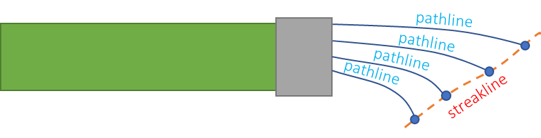
Consider fluid starting to come out of a garden hose as the faucet is turned on. The flow may start weakly and then climb until it levels off at the steady state value. Below is a diagram of such a situation (inspired by the lecture from the Cowan Academy). The individual pathlines are quite different and the time the fluid elements came through the outlet of the hose are different. But their motion is stopped at a common time and the line joining them is the streakline. It is particularly useful in that it represents an experiment that can be performed and measured.
Streamlines are best shown using a quiver plot. To be concrete consider the velocity field in 2 dimensions to be given by
\[ V_x= \alpha x \; \]
and
\[ V_y = -\alpha y \; ,\]
where $$\alpha$$ is some real number. A plot of the flow velocity at a grid of points is called a quiver plot and the results for the flow above are (with $$\alpha = 1$$)
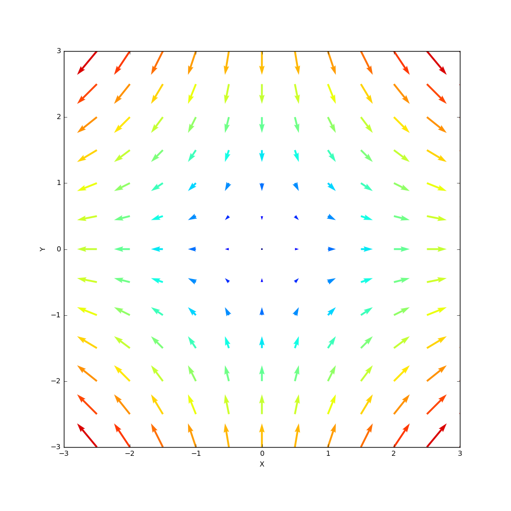
Note that the color of the vectors match their length with red corresponding the largest flow rate and blue the smallest, that they suggest that hyperbolic pattern with flow coming in along the y-axis and flowing along the x-axis, and the is a stagnation point at the origin where the fluid elements there are at rest.
Acheson, in Chapter 1 of Elementary Fluid Dynamics, has a nice problem associated with this flow that accentuates the difference between Lagrangian and Eulerian viewpoints. In the Eulerian viewpoint, the concentration of a pollutant is given by
\[ c(x,y,t) = \beta x^2 y e^{-\alpha t} \; ,\]
which clearly varies in space and time and fades in strength at a given point as time progresses. The question Acheson asks is does the concentration in a fluid element change. To answer, we employ the material derivative, since it follows the flow of a given material element. Taking the material derivative of the concentration gives
\[ \frac{D}{Dt} c(x,y,z) = \frac{\partial c(x,y,t)}{\partial t} + \left( \vec V \cdot \nabla \right) c(x,y,t) \; .\]
The right-hand side of the equation is a set of partial derivatives that, when expanded, is
\[ \partial_t c + \alpha x \partial_x c – \alpha y \partial_y c = -\alpha \beta x^2 y e^{-\alpha t} + 2 \alpha \beta x^2 y e^{-\alpha t} – \alpha \beta x^2 y e^{-\alpha t} = 0 \; . \]
So, the concentration of a fluid element is constant. The reason the concentration decays in strength at a given point is simply that the flow shunts the more polluted elements away from any point and towards infinity. Alternatively, one can use Lagrangian coordinates to describe the flow. The position of a given fluid element is given by
\[ x = X e^{\alpha t} \; \; y = Y e^{-\alpha t} \; , \]
where $$X$$ and $$Y$$ are the x- and y-position of the fluid element at $$t=0$$. In terms of these coordinates the concentration of a fluid element is
\[ c = \beta X^2 e^{-2 \alpha t} Y e^{\alpha t} e^{\alpha t} = \beta X^2 Y \; ,\]
which is manifestly time independent.
With this warm up exercise under our belt, let’s look at an unsteady flow where the difference between streamlines and pathlines becomes obvious.
Consider the flow
\[ V_x = V_{x_0} \; \; V_y = k t \; \]
The quiver plots for two different times are shown here (with $$V_{x_0} = 1$$ and $$k=1$$).
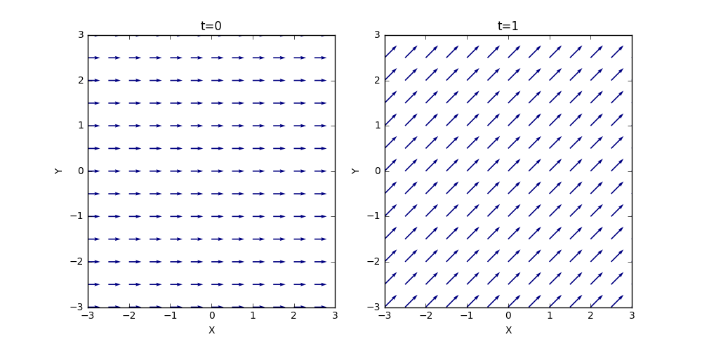
In both cases, the streamlines are straight lines but with a time varying slope, as evidenced by the different slopes at different times.
The pathlines come from integrating
\[ \frac{\partial x}{\partial t} = V_{x_0} \;\; \textrm{and} \;\; \frac{\partial y}{\partial t} = k t \; .\]
Performing the integration and and setting the integration constants ($$x(t=0) = X$$ and $$y(t=0) = Y $$) to zero gives
\[ x(t) = V_{x_0} t \;\; \textrm{and} \;\; y(t) = \frac{1}{2} k t^2 \; .\]
Solving the first equation for $$t$$ and substituting into the second equation gives the geometric path of
\[ y = \frac{1}{2} \frac{k}{V_{x_0}^2} x^2 \; , \]
which shows that the particles follow a parabolic pathline even though the streamlines are always linear.