One of the most confusing aspects of Lagrangian/Hamiltonian mechanics centers on the energy $$E$$ and its relationship to the function $$h$$ (or to the Hamiltonian $$H$$, to which it is closely related). The key questions are, to what extent these two terms can be identified with each other, and which of them is conserved and in which circumstances. The answers have deep implications into the analysis of the possible motions the system supports. The opportunity for confusion arises because there are many different possibilities that show up in practice.

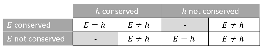
The aim of this and the following columns is to delve into these cases in sufficient detail to flesh out the six logically possible cases that result from $$E$$ being either conserved or not, $$h$$ being either conserved or not, both subject to the possible constraint that $$E=h$$.

Before going into specific analysis of this case or that, it is important to get an overview as to how these various cases result in practice. Central to the variety of possibilities is the notion of generalize coordinates and the application of dynamical constraints.

As discussed in great detail in Classical Mechanics by Goldstein (especially Chapter 1), generalized coordinates are what provide the Lagrangian method with its power by enabling it to rise above Cartesian coordinates and into a frame better adapted to the geometry of the dynamics. For example, central force motion is best described in plane-polar coordinates that not only make the computations easier but also provide a simple method of imposing constraints like, the motion must take place at a fixed radius (e.g., a bead on a loop of wire). The number of generalized coordinates can always match the number of degrees of freedom, a condition that usually can’t be fulfilled in Cartesian coordinates if there are constraints. Generalized coordinates serve as the cornerstone in understanding rigid body motion – the three Euler angles mapping directly to the three degrees of freedom such a body has to move about its center of mass.

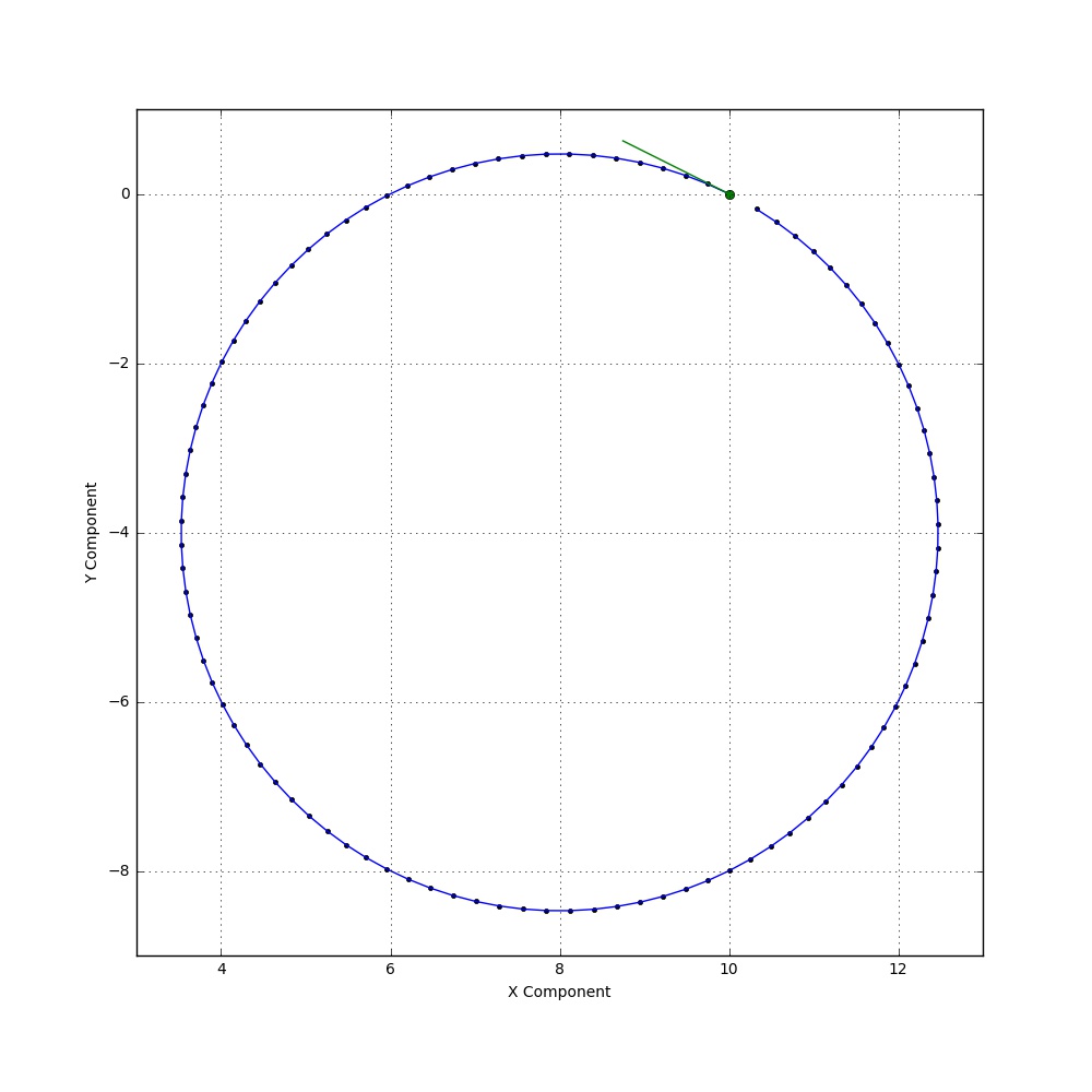
The price for such freedom is that the universe of possible conserved quantities must be enlarged from the obvious ones evident in elementary mechanics to a broader set. This expansion in scope leads to the need to distinguish between the energy $$E$$ and the function $$h$$. One of the most important and famous examples of this is the conservation of the Jacobi constant in the circular-restricted three-body problem.

But, before launching into an analysis that compares and contrasts $$E$$ with $$h$$, it is important to establish some basic results of the Lagrangian method.

The first result is that the Lagrangian equations of motion are invariant under what Goldstein calls a point transformation

\[ q^i = q^i(s^j,t) \; , \]

relating one set of generalized coordinates $$q^i$$ to another $$s^j$$ (note that Cartesian coordinates are a subset of generalized coordinates).

Transformation of the Lagrangian $$L(q^i,t)$$ to $$L'(s^j,t)$$ starts with determining the form of the generalized velocities

\[ {\dot q}^i = \frac{\partial q^i}{\partial s^j} {\dot s}^j + \frac{\partial q^i}{\partial t} \; , \]

($$\dot f \equiv \frac{d}{dt} f$$).

From this relation comes the somewhat counterintuitive ‘cancellation-of-the-dots’ that states

\[ \frac{\partial {\dot q}^i}{\partial {\dot s}^j} = \frac{\partial q^i}{\partial s^j} \; .\]

A needed corollary of the cancellation-of-the-dots results from applying the total time derivative to both sides of the above relation. The right-hand side expands as

\[ \frac{d}{dt} \left( \frac{\partial q^i}{\partial s^j} \right) = \frac{\partial^2 q^i}{\partial s^k \partial s^j} {\dot s}^k + \frac{\partial^2 q^i}{\partial t \partial s^j} \; .\]

Switching the order of partial derivatives (always allowed for physical functions) and regrouping terms gives the right-hand side (noting along the way that $$\partial {\dot s}^k / \partial s^j = 0 $$) as

\[ \frac{\partial}{\partial s^j} \left( \frac{\partial q^i}{\partial s^k} {\dot s}^k + \frac{\partial q^i}{\partial t} \right) = \frac{\partial}{\partial s^j} \frac{d q^i}{d t} \; . \]

The next step is to grind through the equations of motion, which is straightforward if a bit tedious. Start by labeling the Lagrangian that results after the substitution of the point transformation as

\[ L’ (s^j,{\dot s}^j,t ) = L (q^i(s^j),{\dot q}^i(s^j,{\dot s}^j),t ) \; .\]

The coordinate-derivative piece of the equations of motion gives

\[ \frac{\partial L’}{\partial s^j} = \frac{\partial L}{\partial q^i} \frac{\partial q^i}{\partial s^j} + \frac{\partial L}{\partial {\dot q}^i} \frac{\partial {\dot q}^i}{\partial s^j} \; . \]

The velocity derivative piece of the equations of motion gives

\[ \frac{\partial L’}{\partial {\dot s}^j} = \frac{\partial L}{\partial {\dot q^i}} \frac{\partial {\dot q}^i}{\partial {\dot s}^j} \; . \]

Combining these pieces into the Euler-Lagrange equations gives

\[ \frac{d}{dt} \left( \frac{\partial L’}{\partial {\dot s}^j } \right) – \frac{\partial L’}{\partial s^j} = \frac{d}{d t} \left( \frac{\partial L}{\partial {\dot q}^i} \right) \frac{\partial {\dot q}^i}{\partial {\dot s}^j} + \frac{\partial L}{\partial {\dot q}^i} \frac{d}{dt} \left( \frac{\partial {\dot q}^i}{\partial {\dot s}^j} \right) \\ – \frac{\partial L}{\partial q^i} \frac{\partial q^i}{\partial s^j} – \frac{\partial L}{\partial {\dot q}^i} \frac{\partial {\dot q}^i}{\partial s^j} \; .\]

Cancellation-of-the-dots and its corollary tells us that the second and fourth terms on the right-hand side cancel, leaving

\[ \frac{d}{dt} \left( \frac{\partial L’}{\partial {\dot s}^j } \right) – \frac{\partial L’}{\partial s^j} = \left[ \frac{d}{d t} \left( \frac{\partial L}{\partial {\dot q}^i} \right) – \frac{\partial L}{\partial q^i} \right] \frac{\partial q^i}{\partial s^j} \; . \]

Since the original equations of motion are zero and the Jacobian of the point transformation is not, we conclude that

\[ \frac{d}{d t} \left( \frac{\partial L}{\partial {\dot q}^i} \right) – \frac{\partial L}{\partial q^i} = 0 \; , \]

which informs us that the Euler-Lagrange equations are invariant under point transformations. This result is our hunting license to use any coordinates related to Cartesian coordinates by a point transformation to describe a system’s degrees of freedom.

The next result is that the Lagrangian is invariant with respect to the addition of a total time derivative. In other words, the same equations of motion result from a Lagrangian $$L$$ as do from one defined as

\[ L’ = L + \frac{d F(q^i,t)}{dt} \; .\]

The proof is as follows. Applying the Euler-Lagrange operator to both sides of the definition of $$L’$$ gives

\[ \frac{d}{dt} \left( \frac{\partial L’}{ \partial {\dot q}^i } \right) – \frac{\partial L’}{\partial q^i} = \frac{d}{dt} \left( \frac{\partial L}{ \partial {\dot q}^i } \right) – \frac{\partial L}{\partial q^i} + \frac{d}{dt} \left( \frac{\partial}{\partial {\dot q}^i} \frac{dF}{dt} \right) – \frac{\partial}{\partial q^i} \frac{dF}{dt} \;. \]

Invariance of the equations of motion requires the last two terms to cancel. The easiest way to see that they do is to first concentrate on the expansion of the total time derivative of $$F$$ as

\[ \frac{d F}{dt} = \frac{\partial F}{\partial q^j} {\dot q}^j + \frac{\partial F}{\partial t} \; . \]

The expression within the third term above then becomes

\[ \frac{\partial}{\partial {\dot q}^j} \left( \frac{d F}{dt} \right) = \frac{\partial F}{\partial q^i} \; . \]

Cancellation of the last two terms now rests on the recognition that

\[ \frac{d}{dt} \left( \frac{\partial F}{\partial q^i} \right) = \frac{\partial}{\partial q^i} \left(\frac{dF}{dt} \right) \; ,\]

a fact easily established by realizing that the total time derivative is a specific sum of partial derivatives and that partial derivatives commute with each other.

This result allows us to play with the form of the Lagrangian in an attempt to find the simplest or most compact way of describing the motion of the physical system.

Next month’s column will use the general structure of this formalism as a guide to the connection between the energy $$E$$ and $$h$$. The columns in the following months will apply the two results derived here to various physical systems in order to illustrate the various cases for $$E$$ and $$h$$ outlined above.

Action and reaction; Newton’s 3rd law tells us that for every action there is an equal an opposite reaction. Nature, in effect, is a banker whose accounts are carefully balanced according to the principle of double-entry bookkeeping. Modern theories emphasize this point of view by saying that at the fundamental level all interactions are mediated by the exchange of ‘force quanta’ that transfer energy, momentum, and angular momentum. So all is well – or is it?

Often textbooks muddy the water of this ‘simple’ situation by engaging in nuanced discussions and citing exceptions without emphasizing two points. One is that action-reaction is always honored. The second is that it may require careful logic supported by exact experiements to rescue new cases that seem to be the exception.

Now, these nuances and exceptions, which roughly fall into three prototypical classes, are real and need to be addressed. Each is interesting in its own right, helping to illustarte and explore the richness of the action-reaction concept, but the ‘answer’ for each of these cases is always the same – there are degrees of freedom that are being ignored that balance the action-reaction.

Case 1 – Dissipative forces

Friction is one of the earliest examples of what is discussed in which action-reaction seems to be violated. Energy is bled out of the system and the motion eventually comes to a halt. The prototype example is the damped harmonic oscillator. Its equation of motion is given by

\[ m {\ddot x} + \Gamma {\dot x} + k x = 0 \; , \]

with the general solution

\[ x(t) = A e^{-\gamma t} \cos( \omega t + \phi ) \; , \]

with $$\gamma = \Gamma/2m$$ and $$\omega = \sqrt{\Gamma^2/4 m^2 – k/m}$$.

It is natural to ask, where does the energy go? In this model, the energy disappears with no account as to where and how. Of course, the accepted answer is straightfoward enough. The energy goes into heat; into degrees of freedom not directly tracked by this model. There is balance on the action-reaction front. There is a reaction force of the oscillator on the environment and it is this force which transfers the energy to the surroundings.

While this accepted answer is known to virtually everybody who’s taken a physics class, it is worth pausing to consider that it wasn’t neccessarily obvious to those who first grappled with this problem, nor is it obvious to the beginner who is introduced to it. In fact, it is very difficult to find a detailed argument that traces through all of the evidence in a logical fashion. It is simply common knowledge supported by our belief in the balance of action and reaction.

Case 2 – Driving forces

The second case, which is actually closely related to the first, involves a driving force that maintains some aspect of the system. Energy, momentum, and/or angular momentum enter and leave the system without being explicitly tracked. The best example of such a system is the circular restricted three-body problem. There are numerous applications of this model to spaceflight, with many missions exploiting the $$L_1$$ and $$L_2$$ Lagrange points.

In the circular-restricted three-body problem, two massive bodies are in orbit around their common barycenter. This motion honors action-reaction perfectly with the gravitational force between the bodies being equal and opposite. The ‘forced motion’ which breaks action-reaction, takes place in the idealization where a test particle is introduced into the system. The test particle is thought to be so small that its back-reaction on the motion of the two bodies can be ignored. The equation of motion is

\[ \ddot {\vec r} = m_1 \frac{\vec r_1 – \vec r}{|\vec r_1 – \vec r|^3} + m_2 \frac{\vec r_2 – \vec r}{|\vec r_2 – \vec r|^3} \; ,\]

with the motion of the primaries given by

\[ \vec r_1 = m_2 L \left( \cos(\omega t) \hat \imath + \sin(\omega t) \hat \jmath \right) \]

and

\[ \vec r_2 = -m_1 L \left( \cos(\omega t) \hat \imath + \sin(\omega t) \hat \jmath ) \right) \]

and with

\[ \omega = \frac{G(m_1 + m_2)}{L^3} \; . \]

That the motions of $$m_1$$ and $$m_2$$ are set by their interaction with no influence from the test particle is the source of the driving force. So, by construction, the model violates Newton’s third law.

But often treatments of the circular-restricted three-body problem confuse this simple point by dwelling on the conservation of the Jacobi constant. This conservation is clearly an important point as it helps in the understanding of the global properties of the solutions. Nonetheless, discussions about its importance rarely emphasize that while the model violates action-reaction, real physical situations do not. The conservation of the Jacobi constant is a useful tool but it does not actually occur in nature. Rather a close approximation results. While this distinction may seem subtle in theory it is quite important in practice – real physical situations cannot be expected to exactly conserve the Jacobi constant.

Case 3 – Velocity-Dependent Forces

The case of velocity-dependent forces is perhaps the most confusing member of this list. There are two reasons for this. The first is that the physics literature usually employs this term to mean only one kind of velocity-dependent force: the force of magnetism. Second, the force of magnetism cannot be studied without direct analysis of the fields that act as intermediaries. This latter point should be one of clarity in the community when in fact it is often one of confusion.

Case in point, the discussion in Chapter 1 of Goldstein’s Classical Mechanics concerning the weak and strong forms of action-reaction pairs. Goldstein has this interesting point to make about action and reaction

He goes on to say that:

Of course, this is eactly the well-known conservation law discussed in a previous post on Maxwell’s equations. There is no reason to erode the confidence in the reader by the inclusion of quotes around the field angular momentum.

The situation is somewhat relieved by a footnote that attempts to give concrete scenarios. There are two of them and this post will deal with them in turn.

The first part states

which, diagrammitically, looks like

Since there are only two particles, the most economical description has their motion take place in a plane. The parallel velocity vector is

\[ \hat v = \cos(\alpha) \hat \imath + \sin(\alpha) \hat \jmath \]

and the separation vector between them is

\[ \vec r_{12} = \vec r_{1} – \vec r_{2} = \rho \hat \jmath \; .\]

The combined electrostatic and magentic force on particle 1 due to particle 2 is

\[ \vec F_{12} = \frac{q^2}{4 \pi \rho^2} \left[ \mu_0 \hat v \times ( \hat v \times \hat y ) – \frac{1}{\epsilon_0} \hat y \right] \; .\]

Substituting in the form of $$\hat v$$ and simplifing gives

\[ \vec F_{12} = \frac{q^2}{4 \pi \rho^2} \left[ \mu_0 \left( \sin(\alpha) \cos(\alpha) \hat \imath – \sin^2(\alpha) \hat \jmath \right) – \frac{1}{\epsilon_0} \hat y \right] \ ;. \]

Since the only thing that changes in computing the force on particle 2 due to particle 1 is the sign on the relative position vector it is easy to see that

\[ \vec F_{21} = -\vec F_{12} \]

and action-reaction is honored. However, this force is action-reaction in its weak form where the forces don’t lie along the vector joining the two particles. This conclusion is best supported by computing the $$x$$-component of the force

\[ \vec F_{12} \cdot \hat \imath = \frac{q^2}{4 \pi \rho^2} \mu_0 \sin(\alpha) \cos(\alpha) \; , \]

which is zero for only a few isolated angles.

The second part of the footnote states

The scenario here can be pictured as

Now the statement in this footnote is clearly gibberish and it is corrected in the 3rd edition to change ‘nonvanishing force’ to ‘nonvanishing magnetic force’, so we’ll focus solely on magentic force.

From the Biot-Savart law the magnetic force on particle 1 due to particle 2 is

\[ \vec F_{12} = -\frac{\mu_0 q^2 v^2}{4 \pi \rho^2} \hat \imath \times ( \hat \jmath \times \hat \jmath ) = 0 \]

while the force on 2 due to 1 is

\[ \vec F_{21} = \frac{\mu_0 q^2 v^2}{4 \pi \rho^2} \hat \jmath \times ( \hat \imath \times \hat \jmath ) = \frac{\mu_0 q^2 v^2}{4 \pi \rho^2} \hat \imath \neq 0 \; .\]

Clearly action-reaction seems violated but strictly speaking this is not true. What should be emphasized is that there is a ‘third body’ in the mix, the electromagnetic field and that the action-reaction can be restored (although not quite point-wise) by looking for additional degrees of freedom.

The last column presented the general theory of the method of moving frames and the concept of a minimal frame in which the time derivatives of the basis vectors, when expressed in terms of themselves, requires only two parameters rather than the usual 3. Building on that work, this column has a two-fold aim. The first is to apply these techniques to the often-studied space curve of the the twisted cubic. The second aim is to touch base with earlier columns on moving frames, thus relating the nature of the moving frame (whether minimal or not) to the traditional concept of angular velocity and, in the process, shine light on the concept of a minimal frame from a new angle.

The twisted cubic, which is the star in this month’s drama, is defined as a curve in three dimensions given by:

\[ \vec r(t) = t \hat e_x + t^2 \hat e_y + t^3 \hat e_z \; , \]

where the parameter $$t$$ can be regarded as time.

Since they will be needed later, the velocity and acceleration of the twisted cubic are given by

\[ \vec v(t) = \hat e_x + 2 t \hat e_y + 3 t^2 \hat e_z \; \]

and

\[ \vec a(t) = 2 \hat e_y + 6 t \hat e_z \; , \]

respectively.

The twisted cubic, shown in the following figure for the range $$t \in [-2,2]$$, has an unusual shape that is best revealed by projecting it to the three coordinate planes. In the $$x-y$$ plane, the curve’s projection is a simple parabola (i.e. $$y(x) = x^2$$). In the $$x-z$$ plane, the curve’s projection is a simple cubic (i.e. $$z(x) = x^3$$). Nothing amazing here. The interest lies in the projection into the $$y-z$$ plane, where a ‘cusp’ appears when $$t$$ passes through the value of 0.

To apply the method of moving frames, the VBN and RIC coordinate frames will be used. VBN is not minimal and RIC is, so there is a nice opportunity to compare and contrast.

While both frames were discussed in the previous column, it is convenient to reiterate their definitions and to present in detail their derivatives. In this later case, some new results will be presented.

The VBN frame is defined as

\[ \hat V = \frac{\vec v}{|\vec v|} \; ,\]

\[ \hat N = \frac{ \vec r \times \vec v }{ | \vec r \times \vec v | } \;, \]

and

\[ \hat B = \hat V \times \hat N \; .\]

Using the general results derived last time, the derivative of $$\hat V$$ is expressed as

\[ \frac{d \hat V}{dt} = \frac{\vec a}{|\vec v|} – \vec v \left( \frac{\vec v \cdot \vec a}{|\vec v|^3} \right) \; .\]

It will be convenient to define $$\vec L = \vec r \times \vec v$$. Doing so allows for the time derivative of $$\hat N$$ to be compactly written as

\[ \frac{d \hat N}{dt} = \frac{\vec r \times \vec a}{|\vec L|} – \vec L \left( \frac{\vec L \cdot \dot{\vec L}}{|\vec L|^3} \right) \; ,\]

where $$\dot{\vec L} = \vec r \times \vec a$$.

The time derivative of $$\hat B$$ is then given in terms of $$\hat V$$ and $$\hat N$$ and their derivatives as

\[ \frac{d \hat B}{d t} = \frac{d \hat V}{d t} \times \vec N + \vec V \times \frac{d \hat N}{d t} \; .\]

The RIC frame is defined by

\[ \hat R = \frac{\vec r}{|\vec r|} \; ,\]

\[ \hat C = \frac{ \vec r \times \vec v }{ | \vec r \times \vec v | } \; ,\]

and

\[ \hat I = \hat C \times \hat R \; .\]

The time derivative of $$\hat R$$ is

\[ \frac{d \hat R}{dt} = \frac{\vec v}{|\vec r|} – \vec r \left( \frac{\vec r \cdot \vec v}{|\vec r|^3} \right) \; .\]

which is a formula analogous to the one for $$\hat V$$.

Since RIC’s $$\hat C$$ is the same as VBN’s $$\hat N$$, its time derivative is identical with a minor change in symbols.

The time derivative of $$\hat I$$ is given by

\[ \frac{d \hat I}{d t} = \frac{d \hat C}{dt} \times \hat R + \hat C \times \frac{d \hat R}{dt} \; .\]

As discussed in Cross Products and Matrices, the moving frame’s motion can be expressed in terms of classical angular momentum, with the mapping $$\alpha \rightarrow -\omega_z$$, $$\beta \rightarrow \omega_y$$, and $$\gamma \rightarrow – \omega_x$$.

With this mapping in hand, one can see that minimal frames are special in that they only have two non-zero components of their angular velocity. For the twisted cubic, the three components of the VBN angular momentum are

and the three components of the RIC angular velocity are

Note that, in the VBN frame, all three components of the angular velocity are generally non-zero, whereas in the RIC, $$\omega_y$$ is always zero.

Also interesting is the time evolution of the magnitude of the angular velocity, $$|\mathbf{\omega}|$$, in the two frames.

The VBN frame is generally ‘rotating’ more slowly than the RIC frame away from the ‘origin’ but quickly rises above in the vicinity.

To close, it is important to note that minimal frames are not intrinsically better than non-minimal frames. Minimal frames may be more convenient in some contexts and more inconvenient in others, but it is likely that their best use is in analytic models since the amount of work is reduced by a third.

One of the most remarkable things about vectors is also one of the most non-intuitive things – at least judging by how hard it is to teach; namely that the rate of change in a set of vectors can be expressed in terms of the vectors themselves. I think it is hard to relate to because it is typically applied in situation where a set of unit vectors, spanning a space, are moving with respect to a set of fixed vectors. The notion that is hard to accept is that time derivatives of these vectors can be written as linear combinations of the same vectors, even though they are changing. On the surface, it seems like a contradiction where something moving and fluid is expressed in terms of something that is moving as well. A sort of self-referential recipe for confusion. And yet, this is precisely what the method of moving frames does and which has proven very successful.

In a nutshell, the method of moving frames states that the motion of a set of unit vectors $$\left\{\hat e_x, \hat e_y, \hat e_z\right\}$$, which, for example, may be the body axes for a rotating object, can be written as

\[ \frac{d}{dt} \left[ \begin{array}{c} \hat e_x \\ \hat e_y \\ \hat e_z \end{array} \right] = \left[ \begin{array}{ccc} 0 & \alpha & \beta \\ -\alpha & 0 & \gamma \\ -\beta & -\gamma & 0 \end{array} \right] \left[ \begin{array}{c} \hat e_x \\ \hat e_y \\ \hat e_z \end{array} \right] \; .\]

The assymetry of the of pre-multiplying matrix, is a consequence of the unit lengths of each member of the set and their mutual orthogonality. In other words, the orthonormality,

\[ \hat e_i \cdot \hat e_j = \delta_{ij} \; ,\]

of the set leads to the relation

\[ \frac{d}{dt} \left( \hat e_i \cdot \hat e_j \right) = 0 \;. \]

The above relation has two very different outcomes depending on what the indices $$i, j$$ are. If they are identical, then the zero on the right-hand side reflects the unit length of each of the basis vectors. When they are different, the zero reflects the fact that they are perpendicular.

To be concrete, consider the case where $$i=j=x$$. Expanding the derivative in this case leads to the relation that the time-rate-of-change of each unit vector is perpendicular to the unit vector itself:

\[ \frac{d}{dt} \left(\hat e_x \cdot \hat e_x \right) = \frac{d \hat e_x}{dt} \cdot \hat e_x + \hat e_x \cdot \frac{d \hat e_x}{dt} = 2 \hat e_x \cdot \frac{d \hat e_x}{dt} = 0\; .\]

A consequence of this relationship and the fact that the set spans the space is that the time derivative of $$\hat e_x$$must be expressed as

\[\frac{d \hat e_x}{dt} = \alpha \hat e_y + \beta \hat e_z \; , \]

where $$\alpha$$ and $$\beta$$ can be determined as shown below.

Next consider the case where $$i=x$$ and $$j=y$$. A simple expansion yields

\[\frac{d}{dt}\left( \hat e_x \cdot \hat e_y \right) = \frac{d \hat e_x}{dt} \cdot \hat e_y + \hat e_x \cdot \frac{d \hat e_y}{dt} = 0 \; ,\]

from which one can conclude that

\[ \frac{d \hat e_x}{dt} \cdot \hat e_y = – \hat e_x \cdot \frac{d \hat e_y}{dt} \; .\]

The assymetry of the matrix follows immediately.

On the surface of it, the above analysis suggests that three functions, $$\alpha, \beta, \gamma$$ are needed to fully specify the motion of a frame. A deeper analysis shows that there are cases where one of these functions can be set identically to zero. I refer to frames of this sort as being minimal frames.

A minimal frame may arise in two ways, either the particular choice of motion for the frame results in a simplification, or the frame is intrinsically minimal, regardless of how the basis vectors twist and turn.

The interest in this column is the latter case (although the former will be touched upon).

The scenario that will be analyzed is where the basis vectors are defined locally on a curve, typically in terms of the position, $$\vec r(t)$$ and the velocity, $$\vec v(t)$$. Since normalization plays an important rule, a wise approach is to explore how to take derivatives of functions of vector norms in generic terms and then apply them widely and fruitfully.

The prototype function is the norm itself, expressed, in terms of an arbitrary vector $$\vec A$$, as

\[ |\vec A | = \sqrt{ A_x^2 + A_y^2 + A_z^2 } \; .\]

The partial derivative of the norm with respect to one of the components is given by

\[ \frac{\partial |\vec A|}{\partial A_i} = \frac{1}{2} \left( A_x^2 + A_y^2 + A_z^2 \right)^{1/2} \frac{\partial}{\partial A_i} \left( A_x^2 + A_y^2 + A_z^2 \right) = \frac{A_i}{|\vec A|} \; .\]

Unitizing a vector involves dividing by the norm, so the corresponding derivative,

\[ \frac{\partial}{\partial A_i} \frac{1}{|\vec A|} = -\frac{A_i}{|\vec A|^3} \; ,\]

is also handy to have lying around.

From these basic pieces, total time derivatives are constructed from the chain rule as

\[ \frac{d}{dt} |\vec A| = \frac{\partial |\vec A|}{\partial A_i} \frac{d A_i}{dt} = \frac{A_i {\dot A}_i}{|\vec A|} \]

and

\[ \frac{d}{dt} \frac{1}{|\vec A|} = – \frac{A_i {\dot A}_i}{|\vec A|^3} \; .\]

All the needed tools are at our fingertips so let’s dig in.

The most famous minimal frame is the Frenet-Serret, defined by the set

\[ \hat T = \frac{\vec v}{|\vec v|} \; ,\]

\[ \hat B = \hat T \times \hat N \; ,\]

and

\[ \hat N = \frac{d \hat T}{d t} / \left| \frac{d \hat T}{d t} \right | \; \]

By definition, the derivative of $$\hat T$$ is expressed solely in terms of $$\hat N$$, and the Frenet-Serret frame is minimal by construction. It is conventional to rescale the derivatives to express them in terms of arc-length with

\[ \frac{d}{dt} \hat T = \frac{d \hat T}{d s} \frac{ds}{dt} = v \frac{d \hat T}{d s} \]

as the key formula. Once the conversion has been performed, the definition of $$\hat N$$ takes a particularly simple form

\[ \frac{d}{d s} \hat T \equiv \kappa \hat N \;\]

The other derivatives follow suite, giving the well-known Frenet-Serret relations

\[ \frac{d}{d s} \hat N = – \kappa \hat T + \tau \hat B \]

and

\[ \frac{d}{d s} \hat B = -\tau \hat N \; .\]

The Frenet-Serret frame is not the only useful moving frame. Within the field of astrodynamics, there are several moving frames that help in understanding the motion of heavenly and man-made satellites. Two of the most useful are the VBN and RIC frames.

The VBN frame is defined as

\[ \hat V = \frac{\vec v}{|\vec v|} \; ,\]

\[ \hat N = \frac{ \vec r \times \vec v }{ | \vec r \times \vec v | } \;, \]

and

\[ \hat B = \hat V \times \hat N \; .\]

Patterned in concept after the Frenet-Serret frame, VBN frame’s $$\hat V$$ vector is the same as $$\hat T$$. However VBN differs in one essential way. It’s $$\hat N$$ points along the instantaneous angular momentum vector of the trajectory. This means that there is always a roll-angle about $$\hat T \equiv \hat V$$ to bring the two frames into alignment. As a result VBN is not a minimal frame.

The proof of this result starts from the computation of the time derivative of $$\hat V$$ given by

\[ \frac{d \hat V}{dt} = \frac{d}{dt} \frac{\vec v}{|\vec v|} = \frac{\vec a}{|\vec v|} – \vec v \left( \frac{\vec v \cdot \vec a}{|\vec v|^3} \right) \; ,\]

using the formulas derived above.

As a check that the computation was carried through correctly, note that time derivative of $$\hat V$$ is perpendicular to $$\hat V$$ itself:

\[ \frac{d \hat V}{dt} \cdot \hat V = \frac{\vec a \cdot \vec v}{|\vec v|^2} – \vec v \cdot \vec v \left( \frac{\vec v \cdot \vec a}{|\vec v|^4} \right) = 0 \; .\]

The time-derivatives of $$\hat N$$ and $$\hat B$$ are straightforward but tedious and are not needed to demonstrate the frame is non-minimal. All that is needed is to take the scalar product of the time derivative $$\hat V$$ with these vectors and then to use the fact the assymetry of the matrix.

Doing so with $$\hat N$$ yields

\[ \frac{d \hat V}{dt} \cdot \hat N = \frac{\vec a \cdot (\vec r \times \vec v) }{|\vec v||\vec r \times \vec v|} – \vec v \cdot (\vec r \times \vec v) \left( \frac{\vec v \cdot \vec a}{|\vec v|^3 |\vec r \times \vec v|} \right) \; . \]

The second term vanishes by the cyclic property of the triple-scalar product and the first can be transformed using the same rule into

\[ \frac{d \hat V}{dt} \cdot \hat N = \frac{\vec v \cdot (\vec a \times \vec r) }{|\vec v||\vec r \times \vec v|} \; . \]

Only in special cases of central forces, where $$\vec a$$ is parallel to $$\vec r$$ is this derivative zero; generically it is not.

The final step is to replace $$\hat N$$ with $$\hat B$$ in the scalar product. This yields

\[ \frac{d \hat V}{dt} \cdot \hat B = \frac{d \hat V}{dt} \cdot (\hat V \times \hat N) = \hat V \cdot \left(\frac{d \hat V}{dt} \times \hat N \right) \; .\]

Expanding the right-hand side of this relation gives

\[ \frac{d \hat V}{dt} \cdot \hat B = \frac{ \vec v \cdot [\vec a \times (\vec r \times \vec v)] }{ |\vec v|^3 |\vec r \times \vec v |} – \frac{ \vec v \cdot [\vec v \times (\vec r \times \vec v)]}{|\vec v|^5 |\vec r \times \vec v|} \; .\]

The second terms is identically zero as can be seen by expanding using the BAC-CAB rule

\[ \vec v \cdot [\vec v \times (\vec r \times \vec v)] = \vec v \cdot \left[ \vec r (\vec v \cdot \vec v) – \vec v (\vec v \cdot \vec r) \right ] = 0 \; .\]

Using the same technique, one concludes that the first term is generally not zero

\[ \vec v \cdot [\vec a \times (\vec r \times \vec v)] = \vec v \cdot \left[ \vec r (\vec v \cdot \vec a) – \vec v (\vec a \cdot \vec r) \right ] \; ,\]

since, generally, the acceleration need not cause a cancellation (although in the case of a central force $$\vec a \cdot \vec v = 0$$ and VBN is a minimal frame).

The other, commonly-used astrodynamics frame is the RIC frame, defined by

\[ \hat R = \frac{\vec r}{|\vec r|} \; ,\]

\[ \hat C = \frac{ \vec r \times \vec v }{ | \vec r \times \vec v | } \; ,\]

and

\[ \hat I = \hat C \times \hat R \; .\]

Note that $$\hat C$$ is the same as VBN’s $$\hat N$$. The RIC frame is minimal, as can be seen by computing the time derivative of $$\hat C$$,

\[ \frac{d}{dt} \hat C = \frac{ \vec r \times \vec a}{|\vec r \times \vec v|} – \frac{ \vec r \times \vec v}{|\vec r \times \vec v|^3} \left[ (\vec r \times \vec v) \cdot (\vec r \times \vec a) \right] \; , \]

and then forming its scalar product with $$\hat R$$,

\[ \frac{d \hat C}{d t} \cdot \hat R = A (\vec r \times \vec a ) \cdot \vec r + B (\vec r \times \vec v) \cdot \vec r \; ,\]

where $$A$$ and $$B$$ are scalar functions whose form is irrelevant for this discussion.

Exploiting the cyclic property of the triple scalar product gives

\[ \frac{d \hat C}{d t} \cdot \hat R = 0 \; .\]

This means that the time derivative of $$\hat C$$ is proportional only to $$\hat I$$ thus proving that the RIC frame is minimal.

Last month’s column dealt with the transformation of the wave equation under a Galilean transformation. Under this transformation, a wave moving with speed $$c$$ in a medium (e.g. a string or slinky or whatever) itself moving with speed $$v$$ with respect to some observer will be seen by that observer to be moving with speed $$c \pm v$$ depending on direction. To get this result, some clever manipulations had to be made that related a set of mixed partial derivatives in one frame with respect to the other.

It is natural enough to ask if the wave equation admits other transformations and, if so, do any of these represent anything physical. The idea lurking around is special relativity and the famous null result of the Michelson-Morley interferometer. But for the sake of this post, we will assume only simple physics, dictated by symmetry, and will discover that the Lorentz transformation falls out of the mathematical constraints that arise from the wave equation.

The situation is the same as in the previous post, with an observer $${\mathcal O}’$$ seeing the wave generated in the frame of $${\mathcal O}$$.

This time the transformation used will be symmetric in space and time, with the form

\[ x’ = \gamma( x + vt ) \]

and

\[ t’ = \gamma( t + \alpha x) \; .\]

The term $$\gamma$$ is a dimensionless quantity (whose value, at this point, may be unity) while $$\alpha$$ has units of an inverse velocity. Both of them will be determined from the transformation and some simple physical principles.

Assume, as before, that the wave equation as described by $${\mathcal O}$$ is given by

\[ c^2 \frac{\partial^2 f}{\partial x^2} – \frac{\partial^2 f}{\partial t^2} = 0 \; .\]

The transformation of the partial derivative with respect to the spatial variable in the unprimed to the primed frame is obtained through the chain rule

\[ \frac{\partial f}{\partial x} = \frac{\partial f}{\partial x’} \frac{\partial x’}{\partial x} + \frac{\partial f}{\partial t’} \frac{\partial t’}{\partial x} \; , \]

with an analogous relation for the partial derivatives with respect to time.

Using the transformation above gives

\[ \frac{\partial f}{\partial x} = \gamma \frac{\partial f}{\partial x’} + \alpha \frac{\partial f}{\partial t’} \]

and

\[ \frac{\partial f}{\partial t} = \gamma v \frac{\partial f}{\partial x’} + \gamma \frac{\partial f}{\partial t’} \; .\]

The second partial derivatives are obtained in the same way, but because of the transformation, four terms result from the expansion of

\[ \frac{\partial^2 f}{\partial x^2} = \frac{\partial}{\partial x} \left( \gamma \frac{\partial f}{\partial x’} + \alpha \frac{\partial f}{\partial t’} \right) \]

rather than 2 or 3 in the Galilean case considered before.

Assuming that the mixed partials commute, the middle two terms combine to give

\[ \frac{\partial^2 f}{\partial x^2} = \gamma^2 \frac{\partial^2 f}{\partial x’^2} + 2 \gamma^2 \alpha \frac{\partial^2 f}{\partial x’ \partial t’} + \gamma^2 \alpha^2 \frac{\partial^2 f}{\partial t’^2} \; .\]

Likewise, the second partial derivative with respect to time

\[ \frac{\partial^2 f}{\partial t^2} = \frac{\partial}{\partial t} \left( \gamma v \frac{\partial f}{\partial x’} + \gamma \frac{\partial f}{\partial t’} \right) \]

becomes

\[ \frac{\partial^2 f}{\partial t^2} = \gamma^2 v^2 \frac{\partial^2 f}{\partial x’^2} + 2 \gamma^2 v \frac{\partial^2 f}{\partial t’ \partial x’} + \gamma^2 \alpha^2 \frac{\partial^2 f}{\partial t’^2} \; .\]

Substituting these results into the original wave equation leads to a wave equation expressed in $${\mathcal O}’$$’s frame of

\[ c^2 \frac{\partial^2 f}{\partial x^2} – \frac{\partial^2 f}{\partial t^2} = \gamma^2(c^2 – v^2) \frac{\partial^2 f}{\partial x’^2} – \gamma^2 \left(1 – \frac{v^2}{c^2} \right) \frac{\partial^2 f}{\partial t’^2} \\ + 2 \gamma^2(\alpha c^2 – v) \frac{\partial^2 f}{\partial t’ \partial x’} = 0 \; .\]

There is no need to argue the mixed partial derivative into a different form (as was the case in the Galelean case) since a simple selection of

\[ \alpha c^2 – v = 0 \]

eliminates the term entirely. Solving this equation determines the unknown term $$\alpha$$ as

\[ \alpha = \frac{v^2}{c^2} \; ,\]

leaving the wave equation to take the invariant form of

\[ c^2 \frac{\partial^2 f}{\partial x’^2} – \frac{\partial^2 f}{\partial t’^2} = 0 \; .\]

In other words, the speed of the wave is constant regardless of how either the source or the observer move with respect to each other.

The only unknown term, $$\gamma$$, can be determined by the requirement that the transformation be invertible and that the determinant of the matrix be unity. The reason for the first requirement rests with the fact that there is no preferred frame – that the physics described on one frame can be related to the other no matter which frame is picked as the starting point. Failure to impose the second requirement would mean that the physics in one frame could be changed simply by transforming to another frame and then transforming back.

Since the transformation can be written matrix form as

\[ \left[ \begin{array}{c} x’ \\ t’ \end{array} \right] = \left[ \begin{array}{cc} \gamma & \gamma v \\ \gamma \frac{v}{c^2} & \gamma \end{array} \right] \left[ \begin{array}{c} x \\ t \end{array} \right] \]

then the requirement of a unit determinant means

\[ \gamma^2 – \gamma^2 \frac{v^2}{c^2} = 1 \; .\]

Solving for $$\gamma$$ give the famous Lorentz-Fitzgerald contraction

\[ \gamma = \frac{1}{\sqrt{1-v^2/c^2}} \; .\]

Note that in the limit as $$v \rightarrow 0$$, $$\gamma \rightarrow 1$$ and $$\alpha \rightarrow 0$$, thus restoring the Galilean transformation.

Thus only by starting with a symmetry principle that treats space and time on equal footing and some simple physical requirements on the wave equation, we can find a transformation that predicts that the speed of the wave is constant with respect to all observers. This is exactly what is seen in experiments and the resulting transformation is the gateway into the full machinery of special relativity.

Wave motion is ubiquitous; from the sound waves we use to hear, to waves on a string instrument, from water waves in the ocean, to light waves from the nearest lamp. The universe presents countless examples of waving phenomena. And yet wave motion is often difficult to understand. This month’s column discusses an interesting aspect of waves that I had not fully appreciated until I was casually reading through Electricity and Magnetism for Mathematicians: A Guided Path from Maxwell’s Equations to Yang-Mills by Thomas A. Garrity.

Bought on a whim, I thought I might get some insight into how mathematicians see electricity and magnetism, specifically, and physics, in general, from the book. Their perspective is generally quite different from that of physicists, since their focus is mostly on rigor and the machinery (how a conclusion is obtained) rather than the particular physical basis for that conclusion. In the past, I have uncovered some useful nuggets on physics from similar texts.

Well, I didn’t have to wait long to uncover one from Garrity. In his chapter 3 on electromagnetic waves, I found a derivation on the nature of the wave equation under Galilean transformations that I hadn’t seen or, perhaps, hadn’t appreciated before.

Physics textbook discussions of the Galilean transformation of the wave equation carry through the transformation of the partial derivative from one frame to the other. In doing so, a mixed second-order term emerges and the derivations I’ve seen stop there with the statement that Galilean transformations ruin the form of the wave equation. But, as Garrity shows, there is an additional step that one can make, and that one step reveals a lot of structure.

To start, consider the wave equation in one dimension

\[ c^2 \frac{\partial^2 f}{\partial x^2} – \frac{\partial^2 f}{\partial t^2} = 0 \; .\]

As is well known, a function of the form $$f(x \pm ct)$$ is a solution to the wave equation. This is most easily seen by defining $$p_{\pm} = x \pm c t$$ and using the chain rule where each of the space or time derivatives is mapped to derivatives with respect to $$p_{\pm}$$.

The first derivatives are

\[ \frac{\partial f}{\partial x} = \frac{d f}{d p_{\pm}}\frac{\partial p_{\pm}}{\partial x} = \frac{d f}{d p_{\pm}} \]

and

\[ \frac{\partial f}{\partial t} = \frac{d f}{d p_{\pm}}\frac{\partial p_{\pm}}{\partial t} = \pm c \frac{d f}{d p_{\pm}} \; .\]

The second derivatives are

\[ \frac{\partial^2 f}{\partial x^2} = \frac{d}{d p_\pm} \left( \frac{d f}{d p_{\pm}} \right)\frac{\partial p_{\pm}}{\partial x} = \frac{d^2 f}{d p_{\pm}^2} \]

and

\[ \frac{\partial^2 f}{\partial t^2} = \frac{d}{d p_{\pm}} \left( \pm c \frac{d f}{d p_{\pm}} \right)\frac{\partial p_{\pm}}{\partial t} = c^2 \frac{d^2 f}{d p_{\pm}^2} \; .\]

Using this construction, arbitrarily complex waveforms can be constructed without the bother of decomposing them into their Fourier components. For example, the Gaussian pulse

\[ f(x-ct) = e^{-(x-ct)^2} \]

is an exact solution of the wave equation with a pulse height that propagates to the right with a velocity $$c$$.

Now suppose that this pulse is propagated along a long string at rest in the frame of an observer $${\mathcal O}$$ and that it persists for a long period of time (i.e. $$c \, t << L$$), so that it can be properly observed. Further, suppose that that string is aboard a moving train that propagates with velocity $$\pm v$$ with respect to an observer $${\mathcal O}'$$ who watches from the ground. The ground-based observer $${\mathcal O}'$$ should be able to conclude that the pulse propagates at speed $$c \mp v$$, without knowing anything about strings, waves, or calculus. The operative question thus becomes whether or not the wave equation supports that conclusion.

To decide, the behavior of the wave equation under a Galilean transformation is required.

The transformation linking observations made by $${\mathcal O}’$$ to those made by $${\mathcal O}$$ are

\[ x’ = v t + x \]

and

\[ t’ = t \; ,\]

with the inverse transformations given by

\[ x = x’ – v t’ \]

and

\[ t = t’ \; .\]

The strategy consists of using the chain rule to express the derivatives in observer $${\mathcal O}$$’s frame to those in the frame of $${\mathcal O}’$$. The first derivatives are:

\[ \frac{\partial f}{\partial x} = \frac{\partial f}{\partial x’}\frac{\partial x’}{\partial x} + \frac{\partial f}{\partial t’}\frac{\partial t’}{\partial x} = \frac{\partial f}{\partial x’} \]

and

\[ \frac{\partial f}{\partial t} = \frac{\partial f}{\partial x’}\frac{\partial x’}{\partial t} + \frac{\partial f}{\partial t’}\frac{\partial t’}{\partial t} = v \frac{\partial f}{\partial x’} + \frac{\partial f}{\partial t’} \; . \]

The second spatial derivative follows immediately as

\[ \frac{\partial^2 f}{\partial x^2} = \frac{ \partial^2 f}{\partial x’^2} \; .\]

The second time derivative is a bit more complicated and is best handled in steps. Substitute in for the first derivative to get

\[ \frac{\partial^2 f}{\partial t^2} = \frac{\partial }{\partial t} \left( v \frac{\partial f}{\partial x’} + \frac{\partial f}{\partial t’} \right) \; .\]

Treating the term in parentheses as a new function $$f$$, the rule used above applies again and a subsequent expansion and collection of terms arrives at

\[ \frac{\partial^2 f}{\partial t^2} = v^2 \frac{\partial^2 f}{\partial x’^2} + 2 v \frac{\partial^2 f}{\partial x’ \partial t’} + \frac{\partial^2 f}{\partial t’^2} \; .\]

Combining the two derivatives gives the wave equation in the frame of $${\mathcal O}’$$ as

\[ (c^2 – v^2) \frac{\partial^2 f}{\partial x’^2} – 2 v \frac{\partial ^2 f} {\partial x’ \partial t’} – \frac{\partial^2 f}{\partial t’^2} = 0 \; . \]

Note the mixed second-order term; this is exactly where most textbooks stop.

But for a right moving pulse, $$f(x-c\,t)$$, the first derivatives are related by

\[ \frac{\partial f}{\partial x} = \frac{d f}{d p_+} \; ,\]

\[ \frac{\partial f}{\partial t} = -c \frac{d f}{d p_+} \; ,\]

and

\[ c \frac{\partial}{\partial x} = -\frac{\partial}{\partial t} \; .\]

Using this relation eliminates that mixed term. First, using the rules derived above, eliminate the partial derivatives in the unprimed frame in favor of those in the primed frame to get

\[ c \frac{\partial}{\partial x’} = – v \frac{\partial}{\partial x’} – \frac{\partial}{\partial t’} \; .\]

Lastly, eliminate the time derivative in the second-order mixed term in favor of the space derivative to yield

\[ (c^2 – v^2) \frac{\partial^2 f}{\partial x’^2} + 2(c+v)v \frac{\partial f^2}{\partial x’^2} – \frac{\partial^2 f}{\partial t’^2} = 0 \; .\]

The two terms multiplying the second-order space derivative can be combined

\[ c^2 – v^2 + 2cv + 2 v^2 = c^2 + 2cv + v^2 = (c+v)^2 \]

and the wave equation becomes

\[ (c+v)^2 \frac{\partial^2 f}{\partial x’^2} – \frac{\partial^2 f}{\partial t’^2} = 0 \; .\]

From basic notions of relative motion, observer $${\mathcal O}’$$ would expect a right-moving wave moving with speed $$c$$ in $${\mathcal O}$$’s frame to move at speed $$c+v$$ and that is exactly what the wave equation asserts.

For a left-moving pulse ($$f = f(x+ct)$$), the signs change a bit:

\[ \frac{\partial f}{\partial x} = \frac{\partial f}{\partial p_-} \; ,\]

\[ \frac{\partial f}{\partial t} = + c \frac{\partial f}{\partial p_-} \; , \]

and

\[ c \frac{\partial}{\partial x} = \frac{\partial}{\partial t} \; .\]

Similar manipulations then lead to the corresponding relation in $${\mathcal O}’$$

\[ \frac{\partial }{\partial t’} = (c-v) \frac{\partial}{\partial x’} \]

and the analogous wave equation

\[ (c-v)^2 \frac{\partial^2 f}{\partial x’^2} – \frac{\partial^2 f}{\partial t’^2} = 0 \; .\]

Again, basic notions of relative motion demand that observer $${\mathcal O}’$$ sees a left-moving wave with speed $$c$$ in $${\mathcal O}$$’s frame to move at speed $$c-v$$ and that is exactly what the wave equation gives.

This month’s installment focuses on that aspect of plasma dynamics that is strongly analogous with mechanical vibration: plasma oscillations.  Plasma oscillations were first predicted by Paul Langmuir in the 1920s and later observed in vacuum tubes of the day.

These oscillations manifest themselves as cooperative movements in a plasma’s charge distribution that behave sinusoidalally.  The harmonic nature of these deviations from perfect neutrality is basically due to an electrostatic restoring force that, for small amplitudes around equilibrium, is well approximated as quadratic.  Thus the electrostatic restoring force gives rise to a harmonic potential.  The analog with mechanical oscillations is completed with the identification of the electron and ion centers-of-mass velocities with the macroscopic kinetic energy of the mass on the spring.  Plasma oscillations provide strong support for the basic assumptions of electromagnetic theory and a nice example of how mechanics and electrodynamics meet in a physically relevant situation.

The aim here is to derive the formulae for the plasma oscillations for two related cases and then to interpret the results in terms of mechanical vibration with the familiar spring mass system.

Imagine that there is a slab of plasma of length $$\ell_0$$, with cross-sectional area $$A$$ and an initial number density of ions and electrons of $$n_0$$.  Since the condition of quasi-neutrality is in effect, there is no net electric field in any part of the plasma.  Now imagine that due to an outside agency, all of the electrons are displaced by the very small amount of $$\Delta x$$ to the left, leaving a net positive charge on the right and net negative charge on the left, with the thickness of these two ‘non-neutral’ regions is $$\Delta x$$.

How does the plasma respond to this out of equilibrium condition? The first approximation one can make is that the electrons are free to move but the ions are fixed in space.  This corresponds to the physical approximation that the ions have an infinite mass – an approximation that is well supported by the ~2000 – 1 ratio between the mass of a proton and that of an electron.

The electrons will feel a strong restoring force (red arrow) and they will move accordingly.  Since the ions are fixed, they will feel an equal but opposite restoring force (blue arrow) but they will not be able to respond.

The electric field that the electrons and ions will feel, which is most easily obtained from Gauss’s law, is non-zero between the strips of positive and negative charge in an exactly analogous fashion as to the textbook problem on parallel plate capacitors.  The density of ions in the red region is $$n_0$$ and the volume is $$A \Delta x$$.   Since $$\Delta x$$ is small compared to the other dimensions, the electric field is closely approximated as being entirely in the $$x$$-direction and the total flux through a Gaussian surface whose boundaries coincide with the ion region is due strictly to the left and right faces.  The right face flux is exactly zero since the flux from the electrons exactly cancels the flux from the ions.  The left face flux, which is equal to the total flux, is then

\[ \Phi_E = E A \; , \]

which is proportional to the total charge enclosed

\[ \Phi_E = \frac{e n_0 A \Delta x}{\epsilon_0} \; .\]

Equating gives

\[ E= \frac{e n_0 }{\epsilon_0 } \Delta x \; ,\]

which is the usual result for the field between a parallel plate capacitor ($$n_0 \Delta x$$ is the surface charge density).

As the electrons were all displaced uniformly and are experiencing a uniform force, they will move together as a unit, that is to say cooperatively.  The mass of the unit is simply the mass density $$m_e n_0$$ times the volume consumed $$V = A \ell_0$$.  The center of mass of the slab is at $$\ell/2- \Delta x$$ with the corresponding acceleration $$\Delta {\ddot x}$$.  The force on the slab is

\[ F = q_{tot} E = -e n_0 V \frac{e n_0}{ \epsilon_0} \Delta x\]

and the equation of motion of the entire slab is given by:

\[ m_e n_0 V \frac{d^2}{dt^2} \Delta x = -e n_0 V \frac{e n_0} {\epsilon_0} \Delta x \; .\]

Dividing out the common factors gives

\[ \frac{d^2}{dt^2} \Delta x = -\frac{e^2 n_0}{m_e \epsilon_0} \Delta x \; .\]

From this equation we would conclude that, for small displacements, the electron slab would oscillate at the angular frequency

\[ \omega_{pe} = \sqrt{ \frac{e^2 n_0}{m_e \epsilon_0} } \; , \]

which is called the electron plasma frequency (note it is really an angular frequency).

Relaxing the assumption that the ions don’t move makes the analysis somewhat more complicated but only changes the result in a small but crucial way.  The location of both electron and ion centers-of-mass now matter and must be tracked separately.  The picture of their motion is now

Since both species are free to move, the thickness of the exposed electron or ion regions (red and blue) is not determined solely by the movement of their respective centers-of-mass (the ion region pictured above is much larger than $$\Delta x_i$$) .  The total thickness of the exposed regions depends on the relative motion between both centers-of-mass

\[ t = \Delta x_i – \Delta x_e \; .\]

An initial analysis may suggest that there are 8 separate cases: positive or negative variations for each species (2×2) as well as whether the ions are more displaced versus the electrons.  In fact, there are only two cases based on whether $$t$$ is positive (ion strip is on the right) or whether $$t$$ is negative (ion strip is to the left).  The following table shows the 8 variations for $$\ell = 1$$.

The parameters with the ‘min’ designate the leftmost extent of the electron slab ($$e_{min}$$) and the ion slab ($$i_{min}$$).  The parameter $$t_{low} = i_{min} – e_{min}$$.  A negative value, such as in case 1, means that the ion slab has shifted more to the left than the electrons and that the exposed ion region (red) is now on the left while the exposed electron region (blue) is now on the right.  A positive value of $$t_{low}$$ means the converse.  The corresponding parameters at the rightmost side are defined in an analogous fashion.  The color coding assists in visualizing which species is in which location.  Note that the entire table can be summarized by $$\Delta x_i – \Delta x_e$$, whose magnitude and sign match $$t_{low}$$ and $$t_{high}$$.  Also note that the displacements in the table are purely geometric and that the actual dynamic displacements would not shift the total center-of-mass since the only forces in the problem are internal.

The electric field in between the two uncovered charge regions can also be obtained by Gauss’s law, but it is instructive to use the expression for the electric field due to a sheet of charge that and superposition. The electric field due to the ions will have a magnitude of

\[ E_i = \frac{e n_0}{2 \epsilon_0} \left(\Delta x_i – \Delta x_e \right) \]

using the standard result from elementary E&M.

Likewise the electric field due to the electrons will also have the same magnitude $$E_e = E_i$$. Their directions will be the same in the region between them (the neutral plasma) and opposite outside, so that a non-zero field with magnitude $$2 E_i$$ will result only in the middle region. The direction of the field depends on which one is on the right versus the left but it doesn’t matter for the sake of the dynamical analysis.
The equation of motion for each slab is then given by

\[ m_i \frac{d^2}{dt^2} \Delta x_i = -\frac{e^2 n_0}{\epsilon_0} \left(\Delta x_i – \Delta x_e\right) \]

and

\[ m_e \frac{d^2}{dt^2} \Delta x_e = \frac{e^2 n_0}{\epsilon_0} \left(\Delta x_i – \Delta x_e\right) \; . \]

Combining these two equations gives

\[ \frac{d^2}{dt^2} \left( \Delta x_i – \Delta x_e \right) = -\frac{e^2 n_0}{\epsilon_0}\left(\frac{1}{m_e} + \frac{1}{m_i} \right) \left(\Delta x_i – \Delta x_e\right) \]

from which we conclude that the frequency is now

\[ \omega_p^2 = \frac{e^2 n_0}{\epsilon_0}\left(\frac{1}{m_e} + \frac{1}{m_i} \right) = \frac{e^2 n_0}{\epsilon_0 m_e} + \frac{e^2 n_0}{\epsilon_0 m_i} \equiv \omega_{pe}^2 + \omega_{pi}^2 \; .\]

The above analysis has a direct analog in a mechanical system of two unequal masses $$m_1$$ and $$M_2$$ connected by a spring of spring constant $$k$$ and equilibrium length $$\ell_0$$.

Defining the deviations of each mass from the equilibrium positions as

\[ \Delta x_1 = x_1 – x_1^{(0)} \]

and

\[ \Delta x_2 = x_2 – x_2^{(0)} \]

the distance between them takes the form

\[ x_2 – x_1 = x_2^{(0)} + \Delta x_2 – x_1^{(0)} – \Delta x_1 \equiv \ell \; .\]

Combining these two definitions gives

\[ x_2 – x_1 = \Delta x_2 – \Delta x_1 + \ell_0 \equiv \delta \ell + \ell_0 \]

from which the potential follows as

\[ V = \frac{1}{2} k (\ell – \ell_0)^2 = \frac{1}{2} k (\Delta x_2 – \Delta x_1)^2 \; .\]

The Lagrangian takes the form

\[ L = \frac{1}{2} m_1 \Delta \dot x_1^2 + \frac{1}{2} M_2 \Delta \dot x_2^2 – \frac{1}{2} k (\Delta x_2 – \Delta x_1)^2 \; , \]

with the equations of motion becoming

\[ \frac{d}{dt} \frac{\partial L}{\partial \dot x_1} – \frac{\partial L}{\partial x_1} = m_1 \Delta \ddot x_1 + k(\Delta x_2 – \Delta x_1 ) = 0 \]

and

\[ \frac{d}{dt} \frac{\partial L}{\partial \dot x_2} – \frac{\partial L}{\partial x_2} = M_2 \Delta \ddot x_2 – k(\Delta x_2 – \Delta x_1 ) = 0 \]

These equations combine nicely into one expression for the dynamics of the change in the separation between the two masses

\[ \delta \ddot \ell = -\left( \frac{k}{m_1} + \frac{k}{M_2} \right) \delta \ell \; , \]

which immediately tells us that the frequency of the oscillations is given by

\[ \omega^2 = k \left(\frac{1}{m_1} + \frac{1}{M_2} \right) = \omega_1^2 + \omega_2^2 \; .\]

In the limit as $$ M_2 \rightarrow \infty $$, the equation of motion simplifies to

\[ \delta \ddot \ell + \frac{k}{m_1} \delta \ell = 0 \; ,\]

with frequency of

\[ \omega^2 = \frac{k}{m_1} = \omega_1^2 \; .\]

Thus there is a perfect analogy between the two pictures and the cooperative motion of the electrons and ions within the plasma can be interpreted in strictly mechanical terms.

Starting with this installment, the focus shifts from the collective phenomenon of waves in cold plasma to the analysis of single particle motion of a charged particle under the influence of given maagnetic and electric fields. In this column, the motion in a fixed magnetic field will be analyzed. This is the most basic type of motion for plasmas and is almost always treated in the early chapters of plasma textbooks. Oddly enough, it is almost always presented in a cumbersome fashion and the cited ‘exact analytic’ solutions are usually incomplete or inaccurate. The major reason for this situation seems to be the fact that the analytic solutions are of little use in plasma physics. Nonetheless, from a pedagogical point-of-view this disconnect is a problem that should be addressed. This column is devoted to just such an aim.

The starting point is the Lorentz force law from which we obtain the equation of motion

\[ m \frac{d}{dt} \vec v = q \left( \vec E + \vec v \times \vec B \right) \; ,\]

subject to the initial conditions $$\vec r(t=0) \equiv \vec r_0$$ and $$\vec v(t=0) \equiv \vec v_0$$.

The textbook first case assumes that $$\vec E = 0$$, $$\vec B = B \hat z$$, and that the initial conditions are non-zero only in the $$x-y$$ plane. Plugging all these assumptions in yields the two equations of motion
\[ {\dot v}_x = \omega_g v_y \]

and

\[ {\dot v}_y = – \omega_g v_x \; ,\]

where the gyrofrequency is defined as

\[ \omega_g = \frac{q B}{m} \; .\]

Most textbook then try to solve these equations in rather clumsy fashion or they pass over the solution and cite analytic solutions that are incomplete or inaccurate. These will be discussed in detail below.

A much better way to solve these equations is to actually employ the standard mathematical way of solving coupled initial value problems using the fundamental matrix. The technique starts with a rewriting of the equations of motion in matrix form

\[ \frac{d}{dt} \left[ \begin{array}{c} v_x \\ v_y \end{array} \right] = \omega_g \left[ \begin{array}{cc} 0 & 1 \\ -1 & 0 \end{array} \right] \left[ \begin{array}{c} v_x \\ v_y \end{array} \right] \; .\]

The formal solution is given by
\[ \left[ \begin{array}{c} v_x \\ v_y \end{array} \right] (t) = e^{\omega_g A t} \left[ \begin{array}{c} v_{x0} \\ v_{y0} \end{array} \right] \; , \]

with the matrix

\[ A = \left[ \begin{array}{cc} 0 & 1 \\ -1 & 0 \end{array} \right] \; .\]

The matrix exponetial term is easily computed once realizes that $$A$$ squares to

\[ A^2 = \left[ \begin{array}{cc} -1 & 0 \\ 0 & -1 \end{array} \right] \; , \]

which is proportional to the unit matrix.

This is convenient since the power series form of the matrix exponential separates into two terms, each of which converges to a trigonometric function

\[ e^{\omega_g A t} = \cos (\omega_g t) 1 + \sin (\omega_g t) A \; ,\]

where $$1$$ is the $$2 \times 2$$ unit matrix.

Expansion of the fundamental matrix in terms of components results in

\[ e^{\omega_g A t} = \left[ \begin{array}{cc} \cos(\omega_g t) & \sin(\omega_g t) \\ -\sin(\omega_g t) & \cos(\omega_g t) \end{array} \right] \; .\]

Solutions to the initial value problem, in terms of initial conditions, are

\[ v_x(t) = v_{x0} \cos(\omega_g t) + v_{y0} \sin(\omega_g t) \]

and

\[ v_y(t) = -v_{x0} \sin(\omega_g t) + v_{y0} \cos(\omega_g t) \; .\]

To get the particle trajectories, one must then integrate these expressions with respect to time. There are two different ways of doing this and the choice between them is governed mostly by taste.

The first way is to perform a definite integration of both sides between $$t_0$$ (taken, for convenience, to be zero) and current time $$t$$:

\[ \int_{0}^{t} d x = \int_{0}^{t} \; dt’ \; \left( v_{x0} \cos(\omega_g t’) + v_{y0} \sin(\omega_g t’) \right) \; .\]

Explicitly computing the integrals gives

\[ x(t) – x_0 = \left. \frac{v_{x0}}{\omega_g} \sin(\omega_g t’) \right|_{0}^{t} – \left. \frac{v_{y0}}{\omega_g} \cos(\omega_g t’) \right|_{0}{t} \; ,\]

which simplifies to

\[ x(t) = x_0 + \frac{v_{y0}}{\omega_g} + \frac{v_{x0}}{\omega_g} \sin(\omega_g t) – \frac{v_{y0}}{\omega_g} \cos(\omega_g t) \; .\]

In the second method, the integrals are treated as indefinite and a single constant of integration results, giving

\[ x(t) – A = \frac{v_{x0}}{\omega_g} \sin(\omega_g t) – \frac{v_{y0}}{\omega_g} \cos(\omega_g t) \; .\]

The value of

\[ A = x_0 + \frac{v_{y0}}{\omega_g} \]

is then obtained from the initial conditions, resulting in exactly the same result.

For completeness, the result for the motion in the $$y$$ direction is

\[ y(t) = y_0 – \frac{v_{x0}}{\omega_g} + \frac{v_{x0}}{\omega_g} \cos(\omega_g t) + \frac{v_{y0}}{\omega_g} \sin(\omega_g t) \]

Interestingly, of the various textbooks examined in the field, none solve for the particle motion in the way above nor do they cite a functional form for the particle motion so derived. The most common way of tackling the equation of motion is exemplified by the treatment in Baumjohann and Treumann. They differentiate the equations once to decouple them thus arriving at

\[ {\ddot v}_x = -\omega_g^2 v_x \]

and

\[ {\ddot v}_y = -\omega_g^2 v_y \; .\]

This form has a two-fold disadvantage. First, the gyrofrequency $$\omega_g$$ appears squared here, thus losing all notion that particles of different signs in charge gyrate in different directions. Second, the second-order nature of these equations implies that there needs to be two constants of integration for the velocity evolution and a corresponding additional two for the particle motion, when, in fact, Newton’s laws require only four constants total. They fumble at with tis a bit in switching back and forth between the gyrofrequency having a sign and being the absolute value. In addition, they cite the solution to the particle equations as

\[ x – x_0 = r_g \sin( \omega_g t ) \]

and

\[ y – y_0 = r_g \cos( \omega_g t ) \; ,\]

with

\[ r_g \frac{v_{\perp}}{|\omega_g|} \; .\]

Chen tackles the equations similarly, deriving the velocity double-dot form before presenting the solution for the particle motion of

\[ x – x_0 = -i e^{-\omega_g t} \]

and

\[ y – y_0 = \pm e^{-\omega_g t} \; ,\]

which become, upon taking the real part,

\[ x – x_0 = r_g \sin( \omega_g t ) \]

and

\[ y – y_0 = \pm r_g \cos( \omega_g t ) \; .\]

He make no mention as to when to use the two different signs.

In order to see that the solution is derived in this column is correct, a numerical simulation of the equations of motion was implemented in Python, using the IPython/Jupyter framework with numpy and scipy extensions. The figures below show the initial conditions – initial position (green dot) and initial velocity (green line) – and the resulting motion from the numerical integration (blue line) with the analytic solution (red and black dot for positive and negative charge).

Positive Charge

Negative Charge

The agreement is excellent, showing the necessity of the ‘extra’ terms here derived. Also note that the sense of rotation is opposite for the negative charge compared to the positive one.

In tha last installment, the structure of plasma waves propagating along the local magnetic field direction were derived and analyzed. This column is mostly focued on the similar type of analysis for the case of waves propagating perpendicular to the local magnetic field. Along the way, a specific point that was glossed over the in the last analysis will be explored more fully. There are two reasons for this. The first is strictly the desire for these columns to be as complete as possible and a subsequent reading of the last piece as a refresher for this one showed a deficit. The second reason is that the analysis for the perpendicular case requires that point.

As before, the central relationship is the tangent form of the dispersion relation

\[ \tan^2 \theta = -\frac{P(n^2-R)(n^2 – L)}{(Sn^2 – RL)(n^2 – P)} \; , \]

where $$\theta$$ is the angle between the direction of wave propagation and the magnetic field, $$n$$ is the index of refraction, and the terms $$S$$, $$P$$, $$R$$, and $$L$$ are

\[ S = 1 – \sum_s \frac{\omega_{ps}^2}{\omega^2 – \omega_{cs}^2} \; ,\]

\[ P = 1 – \sum_s \frac{\omega_{ps}^2}{\omega^2} \; ,\]

\[ R = 1 – \sum_s \frac{\omega_{ps}^2}{\omega(\omega+\omega_{cs})} \; ,\]

and

\[ L = 1 – \sum_s \frac{\omega_{ps}^2}{\omega(\omega-\omega_{cs})} \; ,\]

respectively.

Perpendicular propagation is obtained by setting $$\theta = \pi/2$$. Since the tangent diverges at $$\pi/2$$, the appropriate dispersion relations result when the denominator goes to zero (i.e. the expression has a pole). The poles of the tangent form of the dispersion relation occur at

\[ n^2 = \frac{RL}{S} \]

and

\[ n^2 = P \; .\]

It is interesting to note that, unlike, the parallel propagation case, there are only two dispersion relations rather than three. Finding the eigenvectors leads to a subtle point that was glossed over in the last column. The intent here is to perform the computation in the proper amount of detail and then to explain why the gloss was permissible in the case of parallel propagation.

To determine the corresponding eigenvectors, it is conceptually most clean to go back to the defining equation for the dispersion tensor, which is given by:

\[ \left( \left( {\vec n}^{\times} \right)^2 + \overleftrightarrow{K} \right) \left[ \begin{array}{c} E_x \\ E_y \\ E_z \end{array} \right] = 0 \; , \]

with

\[ \overleftrightarrow{K} = \left[ \begin{array}{ccc} S & -i D & 0 \\ i D & S &0 \\ 0 & 0 & P \end{array} \right] \; ,\]

and

\[\left( {\vec n}^{\times} \right)^2 = \left[ \begin{array}{ccc} -n^2 \cos^2 \theta & 0 & n^2 \sin \theta \cos \theta \\0 & -n^2 & 0 \\n^2 \sin \theta \cos \theta & 0 & -n^2 \sin ^2 \theta \end{array} \right] \; .\]

When the direction of propagation is perpendicular, then $$\theta = \pi/2$$, and the first term becomes

\[\left( {\vec n}^{\times} \right)^2 = \left[ \begin{array}{ccc} 0 & 0 & 0 \\0 & -n^2 & 0 \\0 & 0 & -n^2 \end{array} \right] \; .\]

The resulting three equations for the electric field are:

\[S E_x – i D E_y = 0 \; ,\]

\[i D E_x + S E_y = n^2 E_y \; , \]

and

\[ P E_z = n^2 E_z \; . \]

The first equation can be solve to express $$E_x$$ in terms of $$E_y$$ as:

\[ E_x = \frac{i D}{S} E_y \, \]

independent of the actual dispersion relation. The solutions of the other two equations, however, depends intimately on the particulars of the dispersion relation.

For the case where $$n^2 = P$$, the $$y$$-equation becomes

\[ \left( S^2 – D^2 – PS \right) E_y = 0 \; , \]

for which the only solution is $$E_y = 0$$, since $$S^2 – D^2 – PS \neq 0$$. The third equation becomes

\[ P E_z = P E_z \; ,\]

which is satisfied with $$E_z$$ being assigned any value $$E_0$$. The corresponding eigenvector

\[ \left[ \begin{array}{c} 0 \\ 0 \\ P \end{array} \right] \]

is aligned along the magnetic field while its direction of propagation is in the plane perpendicular. This is known, according to Gurnett and Bhattacharjee as the ordinary mode. Note that its frequency can be arbitrary unlike the $$P$$ mode in the parallel case.

In contrast, in the case where $$n^2 = RL/S$$, the $$y$$-equation

\[ \left( S^2 – D^2 – RL \right) E_y = 0 \]

has a non-trivial solution since

\[ S^2 – D^2 = RL \]

is an identity. And so the equation is satisfied with $$E_y$$ being assigned any value $$E_0$$. The $$z$$-equation

\[ P E_z = RL/S E_z \]

can only be satisfied by $$E_z = 0$$. The corresponding eigenvector is

\[ \left[ \begin{array}{c} \frac{i D}{S} E_0 \\ E_0 \\ 0 \end{array} \right] \; . \]

This wave mode has its electric field in the $$x-y$$ plane, meaning that it has components neccessarily along and perpendicular to the direction of propagation. The parallel component yields an electrostatic piece while the perpendicular component yields an electromagnetic one. In addtion, its magnitude is no longer independent of the local magnetic field, as was the other cases examine up to this point. The dependence on magetic field strength comes from the $$S$$ and $$D$$ terms that scale $$E_x$$. This wave is termed extraordinary and leads to the hybrid resonances that are discussed at length in Section 4.4.2 of Gurnett and Bhattacharjee.

One last note before closing out this column. Last month, a seemingly simpler way was presented to find the eigenvectors for wave propagation parallel to the local magnetic field. The reason for the shortcut used was that when $$\theta = 0$$

\[\left( {\vec n}^{\times} \right)^2 = \left[ \begin{array}{ccc} -n^2 & 0 & 0 \\0 & -n^2 & 0 \\ 0 & 0 & 0 \end{array} \right] \; .\]

The basic equation

\[ \left( \left( {\vec n}^{\times} \right)^2 + \overleftrightarrow{K} \right) \left[ \begin{array}{c} E_x \\ E_y \\ E_z \end{array} \right] = 0 \; \]

becomes

\[ \left[ \begin{array}{ccc} S & -i D & 0 \\ i D & S &0 \\ 0 & 0 & P \end{array} \right] \left[ \begin{array}{c} E_x \\ E_y \\ E_z \end{array} \right] = \left[ \begin{array}{ccc} n^2 & 0 & 0 \\0 & n^2 & 0 \\ 0 & 0 & 0 \end{array} \right] \left[ \begin{array}{c} E_x \\ E_y \\ E_z \end{array} \right] \; ,\]

which is a basic eigenvalue problem for $$\overleftrightarrow{K}$$ and this is why the last column used a simple method for finding only its eigenvectors.

The last column established the basic equations describing waves in cold magnetized plasma and derived some of the general results that can be deduced without finding explicit solutions. This column begins the detailed examination of the explicit solutions that are supported.

The central relationship for this analysis is the tangent form of the dispersion relation

\[ \tan^2 \theta = -\frac{P(n^2-R)(n^2 – L)}{(Sn^2 – RL)(n^2 – P)} \; , \]

where $$\theta$$ is the angle between the direction of wave propagation and the magnetic field, $$n$$ is the index of refraction, and the terms $$S$$, $$P$$, $$R$$, and $$L$$ are

\[ S = 1 – \sum_s \frac{\omega_{ps}^2}{\omega^2 – \omega_{cs}^2} \; ,\]

\[ P = 1 – \sum_s \frac{\omega_{ps}^2}{\omega^2} \; ,\]

\[ R = 1 – \sum_s \frac{\omega_{ps}^2}{\omega(\omega+\omega_{cs})} \; ,\]

and

\[ L = 1 – \sum_s \frac{\omega_{ps}^2}{\omega(\omega-\omega_{cs})} \; ,\]

respectively.

Selecting a particular value of $$\theta$$ sets the propagation of the wave relative to the magnetic field and constrains the dispersion relation. There are three cases to examine: 1) parallel propagation, 2) perpendicular propagation, and 3) oblique propagation. This column will focus on parallel propagation.

In this case the wave moves along the magnetic field and $$\theta = 0$$. Since $$\tan \theta = 0$$, the propagation modes can be read off of the tangent form by simply finding the zeros of the right-hand side. Doing so yields

\[ P = 0 \; ,\]

\[ n^2 = R \; ,\]

and
\[ n^2 = L \; .\]

While the dispersion tensor

\[ \overleftrightarrow{D}(\vec n, \omega) = \left[ \begin{array}{ccc} S-n^2 & -i D & 0 \\ i D & S-n^2 &0 \\ 0 & 0 & P \end{array} \right] \; .\]

was useful for getting the characteristic equation, the matrix that gives the eigenvectors is the dielectric tensor (since $$n^2$$, in this case, is essentially the eigenvalue – at least for $$x$$ and $$y$$). The dielectric tensor’s form is

\[ \overleftrightarrow{K} = \left[ \begin{array}{ccc} S & -i D & 0 \\ i D & S &0 \\ 0 & 0 & P \end{array} \right] \; ,\]

where $$D = \frac{1}{2}( R – L )$$.

A simple analysis shows that the eigenvector corresponding to $$P=0$$ must have the form

\[ \vec E_{P} = \left[ \begin{array}{c} 0 \\ 0 \\ E_{P} \end{array} \right] \; ,\]

where $$E_P$$ is arbitrary.

This mode corresponds to a longitudinal wave at a frequency equal to $$\pm \omega_p$$, the combined plasma frequency of the system:

\[ P = 0 \Rightarrow \omega^2 = \sum_s \omega_{ps}^2 \; .\]

Since the wave is longitudinal it can’t be electromagnetic in origin and is, instead, associated with electrostatic fluctuations of the charge density along the magnetic field direction.

The eigenvectors for the other two modes require a bit more work but it is obvious that the corresponding eigenvectors can only have non-zero components along the $$x$$- and $$y$$-directions. Hence the structure of the wave is transverse, with the wave’s electric and magnetic fields perpendicular to the external magnetic field. Using wxMaxima, the eigenvector/eigenvalue pairs are given by:

\[ S + D = R: \left[ \begin{array}{c} 1 \\ i \\ 0 \end{array} \right] \]

and

\[ S – D = L: \left[ \begin{array}{c} 1 \\ -i \\ 0 \end{array} \right] \; .\]

The difference in the signs of the imaginary components correspond to the differences in handedness (hence the symbols $$R$$ and $$L$$ for right-handed and left-handed, respectively).

The usual convention for pulling out the handedness comes from multiplying the eigenvector by the time evolution $$e^{-i\omega t}$$ and taking the real part. For the $$R$$-mode, this process results in time dependence of

\[ E_x = E_0 \cos(\omega t) \]

and

\[ E_y = E_0 \sin(\omega t) \; ,\]

which shows that the electric field rotates in a counter-clockwise or right-handed fashion.

For the $$L$$-mode, the sign on the $$y$$-term causes the rotation to be clockwise or left-handed.

As Gurnett and Bhattacharjee point out, further proof that the modes are electromagnetic comes from noting that Fourier version of Faraday’s law gives a non-zero magnetic field

\[ \vec B = \vec k \times \vec E / \omega \; . \]

They further point out that since the wave is transverse then there are no charge fluctuations since Gauss’s law (in Fourier space) reads

\[ \rho = \epsilon_0 i \vec k \cdot \vec E = 0 \; . \]

Having specified the basic nature of these transverse waves, the final step is to say something about their specific dispersion relations.

There are three regimes to consider: 1) high frequency, 2) low frequency, and 3) intermediate frequencies.

High frequency

The high-frequency behavior of both modes is easy to determine. The limit of the corresponding dispersion relations as $$\omega \rightarrow \infty$$ is

\[ \lim_{\omega \rightarrow \infty} R = \lim_{\omega \rightarrow \infty} \left( 1 – \sum_s \frac{\omega_{ps}^2}{\omega(\omega+\omega_{cs})} \right) = 1 \; ,\]

and

\[ \lim_{\omega \rightarrow \infty} L = \lim_{\omega \rightarrow \infty} \left( 1 – \sum_s \frac{\omega_{ps}^2}{\omega(\omega-\omega_{cs})} \right) = 1 \; .\]

In this limit, both modes have $$n^2 = 1$$, which corresponds to free space propagation. Physically, this means that the plasma, composed of massive particles, is unable to respond at the rate the electromagnetic wave is oscillating at and the medium become transparent.

Low frequency

The low-frequency behavior of the two modes is a bit more subtle and are not tackled directly since the $$\omega(\omega \pm \omega_{cs})$$ term in the denominator is difficult to determine. Instead, the best approach is to take the limit of $$S$$ and $$D$$ and then to infer the limits for $$R$$ and $$L$$.

The limit of $$S$$ is

\[ \lim_{\omega \rightarrow 0} S = \lim_{\omega \rightarrow 0} \left( 1 – \sum_s \frac{\omega_{ps}^2}{\omega^2 – \omega_{cs}^2} \right) = 1 + \frac{\omega_{ps}^2}{\omega_{cs}^2} \; .\]

The limit of $$D$$

\[ \lim_{\omega \rightarrow 0} D = \lim_{\omega \rightarrow 0} \left( 1 – \sum_s \frac{\omega_{cs} \omega_{ps}^2}{\omega(\omega^2 – \omega_{cs}^2)} \right) \]

is a bit more involved. In this limit $$\omega^2 – \omega_{cs}^2 = -\omega_{cs}^2$$ and the term can be simplified to

\[ \lim_{\omega \rightarrow 0} \left( 1 + \frac{1}{\omega} \sum_s \frac{\omega_{ps}^2}{\omega_{cs}} \right) \; .\]

The next step is to examine the last term in detail. Expanding leads to

\[ \sum_s \frac{\omega_{ps}^2}{\omega_{cs}} = \sum_s \frac{n e^2}{m_s \epsilon_0} \frac{m_s}{q_s B} = \frac{1}{\epsilon_0 B} \sum_s n q_s = 0 \; , \]

where the requirement of neutrality is used in the last step.

Thus the low-frequency limit of $$D$$ is zero. From this result immediately follows that the low-frequency limits of $$R$$ and $$L$$ are the same as for $$S$$. This limit is fairly common and is defined as the Alfven index of refraction

\[ n_A^2 = 1 + \sum_s \frac{\omega_{ps}^2}{\omega_{cs}^2} \; .\]

Intermediate Frequencies

At intermediate frequencies the index of refraction departs from the low and high frequency limits and can do two very interesting things. First, near either the electron or cyclotron frequency, the $$R$$ or $$L$$ modes can enter into resonance with the electrons or the ions, respectively. Because the cyclotron frequency depends on the sign of the charge, the species interact with the two modes very differently. The right-hand mode can preferentially interact with the electrons near the electron cyclotron frequency. When this happens the index of refraction diverges to positive infinity as approached from below and diverges to negative infinity as approached from above. This last obseravation means that the wave cannot propagate until in the region from the negative regime to the cutoff frequency where $$n^2 > 0$$. Similar bevaior occurs for the $$L$$ mode with the ions with as many cutoffs and resonances as their are species.

The cutoff frequencies correspond to either $$R=0$$ or $$L=0$$. Since ion motion can be ignored at frequencies near the electron cycltron frequency, the $$R$$-mode cutoff is

\[ \omega_{R=0} = \frac{|\omega_{ce}|}{2} + \sqrt{\left(\frac{\omega_{ce}}{2}\right)^2 + \omega_{pe}^2} \; . \]