Latest Posts

Scattering: Part 2 – Simulating Trajectories

The last post detailed how specific types of information could be gleaned from the equation of motion for a $$1/r$$ central potential. Three conserved quantities were discovered: the energy, the angular momentum, and the eccentricity vector. In addition, the radial equation, which gives the trajectory’s distance from the scattering center as a function of polar angle along the trajectory, presented itself after a clever manipulation.

This column presents specific techniques and results for modeling individual scattering trajectories for both repulsive ($$\alpha < 0 $$) and attractive ($$\alpha > 0$$) forces.

The first step in calculating specific, individual trajectories is the transformation of the equation of motion from the usual Newton form

\[ \ddot {\vec r} + \frac{\alpha \vec r}{r^3} = 0 \]

into a state space form. The most straightforward method is to use Cartesian coordinates, which yields the coupled first-order equations

\[ \frac{d}{dt} \left[ \begin{array}{c} x \\ y \\ z \\ v_x \\ v_y \\ v_z \end{array} \right] = \left[ \begin{array}{c} v_x \\ v_y \\ v_z \\ -\frac{\alpha x}{r^3} \\ -\frac{\alpha y}{r^3} \\ -\frac{\alpha z}{r^3} \end{array} \right] \; .\]

Numerical integration of the above system results in an ephemeris representation of the trajectory – a listing of discrete times and corresponding position components $$x, y, z$$ and velocity components $$v_x, v_y, v_z$$. Nonlinear combinations of the state will be used to determine the conserved quantities both as a check on the numerical method but also to emphasize the power affording by finding and exploiting conserved quantities.

All of the numerical modeling was done using Python 2.7, numpy, and scipy under the Jupyter notebook format. Matplotlib is used for all of the plots.

The core function used to integrate the equations of motion is

def TwoBody(state,t,params):
    #unpack the state
    x     = state[0]
    y     = state[1]
    z     = state[2]
    vx    = state[3]
    vy    = state[4]
    vz    = state[5]
    
    #unpack params
    alpha = params['alpha']
    
    #define helpers
    r     = sp.sqrt(x**2 + y**2 + z**2)
    q     = alpha/r**3
    
    #state derive
    ds = [vx, vy, vz, -q*x, -q*y, -q*z]
    return ds

Note its structural similarity to the coupled equation above – specifically, the function TwoBody returns the right-hand side of the system of differential equations. The scipy.integrate function odeint, which provides the numerical integration technique, takes this function, arrays specifying the initial conditions and the time span, and any additional arguments that need to be passed. In this case, the additional argument is a Python dictionary that contains the value of $$\alpha$$.

The odeint function returns an array of state values at the times contained in the array that specifies the time span. Together the two arrays comprise the ephemeris of the system.

One additional, useful ingredient is the function conserved_quantities

def conserved_quantities(soln,params):
    pos     = soln[:,0:3]
    vel     = soln[:,3:6]
    r       = np.sqrt((pos*pos).sum(axis=1)).reshape(-1,1) #makes the broadcast shape correct
    E       = 0.5*(vel*vel).sum(axis=1).reshape(-1,1) - params['alpha']/r #other reshape needed to avoid NxN shape for E
    L       = np.cross(pos,vel)
    Ecc     = np.cross(vel,L)/params['alpha'] -  pos/r
    return E, L, Ecc    

that takes the state array and returns arrays corresponding to the energy, the angular momentum vector, and the eccentricity vector. The conserved quantities serve two purposes. The first is that they help make sense out of the jumble of state variables. This was the point of last week’s column. The second is they provide indicators of the goodness of the numerical techniques. If they are not well conserved, then the numerical techniques are not doing what they should.

The first test case run was for the initial conditions

\[ \bar S_0 = \left[ \begin{array}{c} -30 \\ 0.1 \\ 0 \\ 2.25 \\ 0 \\ 0 \end{array} \right] \]

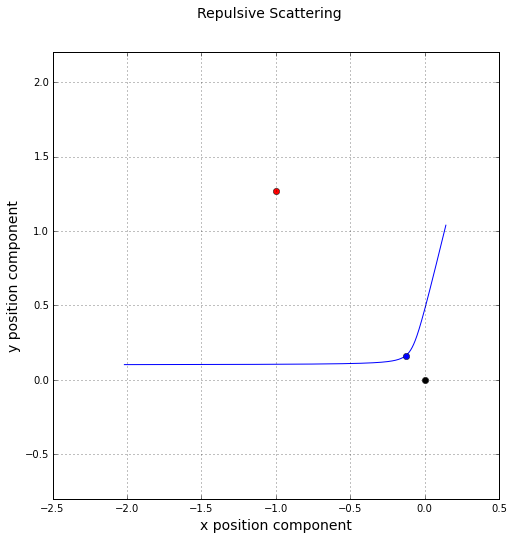
and a value of $$\alpha = -0.4$$. Since $$\alpha < 0 $$, the scattering is repulsive. The resulting trajectory is

repulsive_scattering_trajectory

The black dot indicates the force or scattering center, the blue dot the point of closest approach, and the red dot location of the eccentricity vector.

While the trajectory looks like what we would expect, the is no obvious way to tell, from this figure, whether the ephemeris is correct. Based on the initial conditions, the conserved quantities should be

\[ E = 2.54458 \; ,\]

\[ \vec L = \left[ \begin{array}{c} 0 & 0 & -0.225 \end{array} \right]^T \; ,\]

and

\[ \vec E = \left[ \begin{array}{c} 1 & -1.268958 & 0 \end{array} \right]^T \; .\]

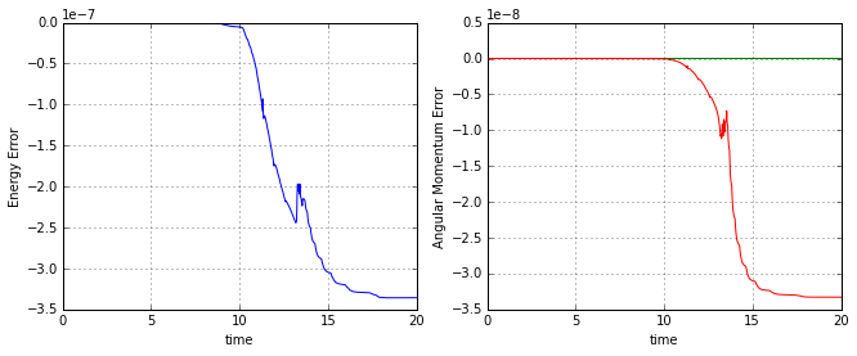
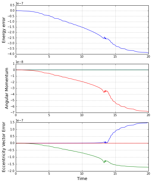
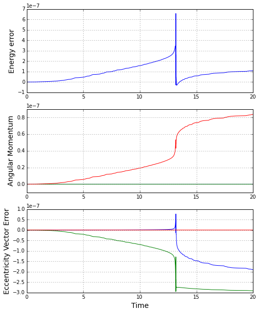
The figure below shows that error in each quantity, where the error is defined as the difference between the instantaneous value and the initial value (e.g. $$\epsilon_E = E(t) – E_0$$).

repulsive_scattering_conserved_quantities

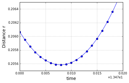
It is clear that the integration does an excellent job of honoring the conservation of the energy, angular momentum, and the eccentricity vector. So now we can believe that the ephemeris is accurate and can test the radial equation. The next figure shows the distance of the trajectory as a function of time in the neighborhood of the closest approach.

repulsive_scattering_closest_approach

From the figure, the closest approach occurs at a distance of $$r = 0.2055838$$. The radial equation, which reads

\[ r(\nu) = \frac{L^2/|\alpha|}{e \cos\nu – 1} \; ,\]

predicts that the closest approach, which occurs at $$\nu = 0$$, of $$r_{CA} = \frac{L^2/|\alpha|}{e-1} = 0.2055838$$.

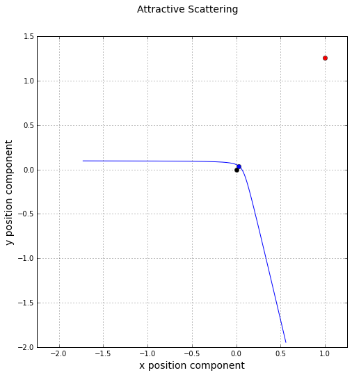
In the same fashion, we can generate a trajectory for $$\alpha = 0.4$$ with the same initial conditions as above. The resulting trajectory is

attractive_scattering_trajectory

Based on the initial conditions, the conserved quantities should be

\[ E = 2.51792 \; ,\]

\[ \vec L = \left[ \begin{array}{c} 0 & 0 & -0.225 \end{array} \right]^T \; ,\]

and

\[ \vec E = \left[ \begin{array}{c} 1 & 1.262292 & 0 \end{array} \right]^T \; .\]

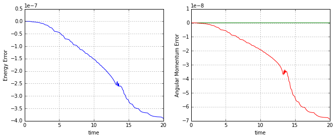
The corresponding figure for the time evolution of the conserved quantities is

attractive_scattering_conserved_quantities

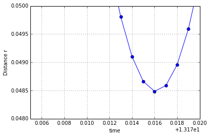
The radial equation predicts $$r_{CA} = 0.04848406$$ compared to a value of $$0.04848647$$ from the plot

attractive_scattering_closest_approach

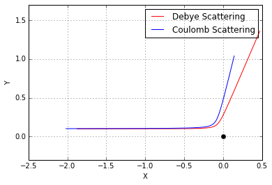
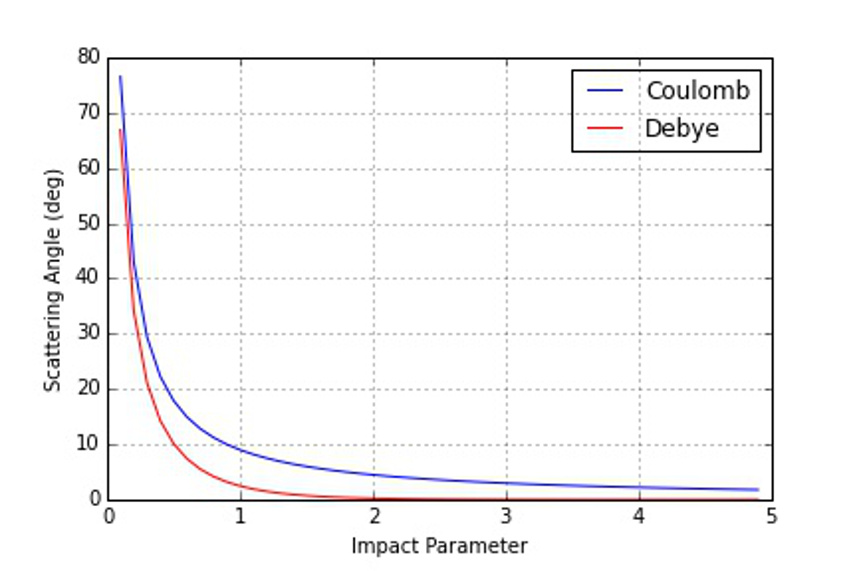
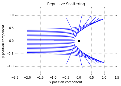
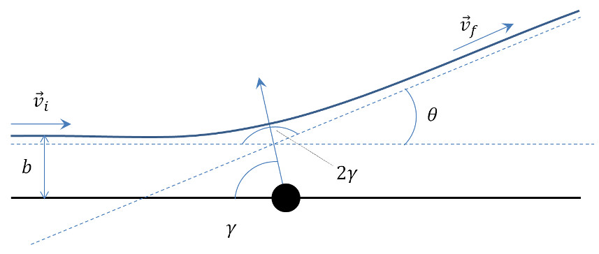
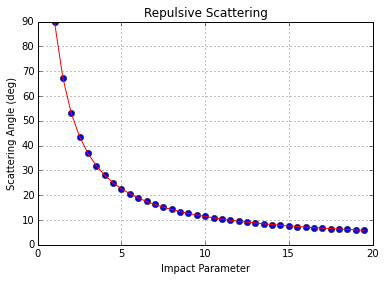
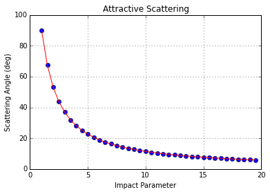
Next week, I’ll be looking at the behavior of an ensemble of trajectories and will be deriving the classical scattering cross section for Rutherford scattering and examining how well the numerical experiments agree.

Scattering: Part 1 – Conserved Quantities

A couple of columns back, I strongly suggested that the definition of the scattering cross section be changed to really reflect its probabilisitic nature and that the geometric picture associated with classical scattering be eliminated. The reasons for that were expressed in the column but what I would like to add in this and subsequent columns is that I am not unsympathetic to the traditional view of the scattering cross section. In fact, I’ve had occasions to use this notion quite often in both professional and hobbyist contexts. So, in the interest of completeness, I am going to be devoting the next four columns to notions associated with scattering within the classical context.

I’ll start with the general theory of scattering from a $$1/r$$-potential. This covers both gravitational and electromagnetic forces, the two forces of classical mechanics.

The equation of motion, quite generally, is

\[ \ddot{\vec r} + \frac{\alpha \vec r}{r^3} = 0 \; .\]

where the sign of $$\alpha$$ determines whether the potential is attractive ($$\alpha > 0$$) or repulsive ($$\alpha < 0$$). Gravitational interactions are always attractive and $$\alpha$$ is usually denoted $$\mu$$ but, for generality, we’ll stick with $$\alpha$$. Now this coupled set of ordinary differential equations is readily solved numerically on just about any computer but the generation of lots of numbers doesn’t help the analysis. A better approach is to interrogate the equations of motion for conserved quantities (click here for the same approach within the context of the Maxwell equations).

Before beginning, it is useful to remind ourselves of some basic identities from many-variable calculus. The first is

\[ \frac{d}{dt} r = \frac{d}{dt} \sqrt{ x^2 + y^2 + z^2 } = \frac{1}{2 \sqrt{ x^2 + y^2 + z^2}} \frac{d}{dt} \left( x^2 + y^2 + z^2 \right) \\ = \frac{ x \dot x + y \dot y + z \dot z}{\sqrt{x^2 + y^2 + z^2}} = \frac{ \vec r \cdot \dot{\vec r} }{r} \equiv \frac{\vec r \cdot \vec v}{r} \; .\]

The second one, which follows directly from the first, is

\[ \frac{d}{dt} \left( \frac{1}{r} \right) = -\frac{ \dot {\vec r} \cdot \vec r}{r^3} \; .\]

Now, the first conserved quantity results from dotting the equation of motion with $$\vec v = \dot {\vec r}$$ to get

\[ \ddot {\vec r} \cdot \vec v + \frac{\alpha \vec r \cdot \vec v }{r^3} \; \]

The first term can be written as a total time derivative since

\[ \frac{d}{dt} \left(\frac{1}{2} \dot {\vec r} \cdot \dot {\vec r} \right) = \dot {\vec r} \cdot \ddot {\vec r} \; .\]

The second term is also a total time derivative as seen from the identities listed above. And so we get our first conserved quantity

\[ E = \frac{1}{2} \dot {\vec r} \cdot \dot {\vec r} – \frac{\alpha}{r} \equiv \frac{1}{2} \vec v \cdot \vec v – \frac{\alpha}{r} \; ,\]

which is the energy of the system.

The next conserved quantity is derived by crossing the equation of motion from the left by $$\vec r$$

\[ \vec r \times \ddot{\vec r} + \frac{\alpha \vec r \times \vec r }{r^3} = 0 \; .\]

Because of the central nature of the force, the last term is identically zero, and the remaining term

\[ \vec r \times \ddot{\vec r} = 0 \]

can be written as a total time derivative

\[ \frac{d}{dt} \left( \vec r \times \dot {\vec r} \right) = 0 \; ,\]

resulting in the conservation of angular momentum

\[ \vec L = \vec r \times \dot {\vec r} = \vec r \times \vec v \; .\]

The final conserved quantity is obtained by crossing the equation of motion from the right by the angular momentum

\[ \ddot {\vec r} \times \vec L + \frac{\alpha \vec r \times \vec L}{r^3} = 0 \; .\]

Since the angular momentum is a conserved quantity, the first term can be rewritten as

\[ \ddot {\vec r} \times \vec L = \frac{d}{dt} \left( \dot {\vec r} \times \vec L \right) = \frac{d}{dt} \left( \vec v \times \vec L \right) \; .\]

The best way to simplify the second term is to recognize that

\[ \frac{d}{dt} \frac{\vec r}{r} = \frac{\vec v}{r} – \frac{\vec r(\vec v \cdot \vec r)}{r^3} = \frac{\vec v r^2 – \vec r(\vec v \cdot \vec r)}{r^3} = -\frac{[\vec r \times (\vec r \times \vec v)]}{r^3} = – \frac{\vec r \times \vec L}{r^3} \; ,\]

where the second-to-last step results from the BAC-CAB rule and the last step is the definition of the angular momentum.

After these manipulations are completed, the resulting total time derivative is

\[ \frac{d}{dt}\left( \vec v \times \vec L – \frac{\alpha \vec r}{r} \right) = 0 \; ,\]

from which we see the conserved quantity

\[ \vec v \times \vec L – \frac{\alpha \vec r}{r} = \vec A \; .\]

This latter vector is known as the Laplace-Runge-Lenz vector.

With all these conserved quantities in place, it is relatively easy to predict certain aspects of the scattering trajectories without solving the equations directly. First, the conservation of angular momentum requires the motion to take place in the plane. As a result, plane-polar coordinates can be used to describe the motion. Since the Laplace-Runge-Lenz vector is conserved and is in the plane perpendicular to the angular momentum, it makes an excellent axis against which to measure the movement of the polar angle $$\nu$$.

\[ \vec A \cdot \vec r = A r \cos \nu \]

The variation of the radius in the plane can then be expressed as a function of $$\nu$$ as follows. Expand the dot product between $$\vec A$$ and $$\vec r$$

\[ \vec A \cdot \vec r = \left( \vec v \times \vec L – \frac{\alpha \vec r}{r} \right) \cdot \vec r = (\vec v \times \vec L) \cdot \vec r – \alpha r \; .\]

Next note, because of the cycle property of the triple-scalar product, that

\[ (\vec v \times \vec L) \cdot \vec r = (\vec r \times \vec v) \cdot \vec L = L^2 \; \]

Equating the two expressions gives

\[ A r \cos \nu = L^2 -\alpha r \; , \]

which can be readily solved to give

\[ r = \frac{L^2 / \alpha}{1 + A/\alpha \cos \nu} \;.\]

Now the interpretation of this equation requires a modest amount of care. If $$\alpha > 0$$, then the above form can immediately be recognized as a conic section with

\[ r = \frac{p}{1+e \cos \nu} \; \; \alpha > 0 ;, \]

where the semi-latus rectum $$p = L^2/\alpha$$ and the eccentricity $$e = A/\alpha$$.

If $$\alpha < 0$$, then we need to multiply the numerator and denominator by $$-1$$ to get \[ r = \frac{L^2 / |\alpha|}{A/|\alpha| \cos \nu – 1} \; , \] from which we get \[ r = \frac{p}{e \cos \nu – 1} \; ,\] where $$p = L^2/|\alpha|$$ and $$e = A/|\alpha|$$. Next week we will analyze individual scattering orbits using these conic equations and the conserved quantities.

Matrices as Vectors

This week’s post will be a short little dive into some of the lesser-known back-waters of linear algebra. As discussed in other posts, a vector space is a rather generic thing with applications to a wide variety of situations that often look quite different than the traditional length-and-direction or column-array pictures that tend to dot the landscape.

One particularly interesting application, if for no other reason than it helps break the fixation that a vector must look like an arrow or a vertically stacked set of numbers is the application to the set of $$2\times2$$ matrices generically denoted as

\[ M = \left[ \begin{array}{cc} a & b \\ c & d \end{array} \right] \; ,\]

where the unspecified numbers $$\left\{a, b, c, d\right\}$$ can be complex.

There are two bases that are nice to use. One is the obvious ‘natural’ basis spanned by vectors

\[ \left| v_1 \right \rangle = \left[ \begin{array}{cc} 1 & 0 \\ 0 & 0 \end{array} \right] \; ,\]

\[ \left| v_2 \right \rangle = \left[ \begin{array}{cc} 0 & 1 \\ 0 & 0 \end{array} \right] \; ,\]

\[ \left| v_3 \right \rangle = \left[ \begin{array}{cc} 0 & 0 \\ 1 & 0 \end{array} \right] \; ,\]

and

\[ \left| v_4 \right \rangle = \left[ \begin{array}{cc} 0 & 0 \\ 0 & 1 \end{array} \right] \; .\]

The matrix $$M$$ is then decomposed, by inspection, to be

\[ \left| M \right \rangle = a \left| v_1 \right \rangle + b \left| v_2 \right \rangle + c \left| v_3 \right \rangle + d \left| v_4 \right \rangle \; .\]

Note the use of Dirac notation for both the basis vectors and the matrix $$M$$. The reason for this notational standard is that it will suggest how to get the components without using inspection, which will be the goal for computer-based decomposition for the second basis discussed below.

The usual way perform decomposition is to provide a natural inner product – bra with ket – so that, for example,

\[ a = \left \langle w_1 \right | \left . M \right \rangle \; .\]

So what is the rule for the bra $$\left \langle w_1 \right |$$? It can’t be the usual complex-conjugate, transpose since the right-hand side of the previous equation is a $$2\times2$$ matrix but the left-hand side is a scalar. Clearly, an added ingredient is needed. And, as will be shown below, that added ingredient is taking the trace.

How then to establish this? Start by assuming the usual definition of the bra; that is let’s ignore the trace piece for the moment and define

\[ \left \langle w_i \right | = \left| v_i \right \rangle^{\dagger} \; i = 1,2,3,4 \; .\]

The basic requirement to impose on the bra-ket relationship is

\[ \left \langle w_i \right | \left . v_j \right \rangle = \delta_{ij} \; . \]

There are 16 possible combinations, but one really only need look at a subset to infer the pattern. For convenience, take $$i=1$$ and let $$j=1,2,3,4$$. The four resulting products are:

\[ \left \langle w_1 \right | \left. v_1 \right \rangle = \left[ \begin{array}{cc} 1 & 0 \\ 0 & 0 \end{array} \right] \; ,\]

\[ \left \langle w_1 \right | \left. v_2 \right \rangle = \left[ \begin{array}{cc} 0 & 1 \\ 0 & 0 \end{array} \right] \; ,\]

\[ \left \langle w_1 \right | \left. v_3 \right \rangle = \left[ \begin{array}{cc} 0 & 0 \\ 0 & 0 \end{array} \right] \; ,\]

and

\[ \left \langle w_1 \right | \left. v_4 \right \rangle = \left[ \begin{array}{cc} 0 & 0 \\ 0 & 0 \end{array} \right] \; .\]

The other 12 products are similar. For each value of $$i$$, the matrix corresponding to $$j=i$$ has a single $$1$$ on the diagonal. Of the three matrices that result from $$j \neq i$$, two matrices are identically zero and the other one has a $$1$$ on the off-diagonal. So to get a single outcome, $$0$$ for $$j \neq i$$ and $$1$$ for $$j=i$$, simply take the trace of the resulting matrix.

This algorithm applies equally well to the second basis, which is one that is based a set of matrices commonly found in modern physics. This basis is spanned by the $$2\times2$$ identity matrix and the Pauli matrices:

\[ \left| I \right \rangle = \left[ \begin{array}{cc} 1 & 0 \\ 0 & 1 \end{array} \right] \; ,\]

\[ \left| \sigma_x \right \rangle = \left[ \begin{array}{cc} 0 & 1 \\ 1 & 0 \end{array} \right] \; ,\]

\[ \left| \sigma_y \right \rangle = \left[ \begin{array}{cc} 0 & -i \\ i & 0 \end{array} \right] \; ,\]

and

\[ \left| \sigma_z \right \rangle = \left[ \begin{array}{cc} 1 & 0 \\ 0 & -1 \end{array} \right] \; .\]

There are two important points to raise here. First, the bra-forms of this basis are identical to the basis itself. Second, each Pauli matrix is trace-free. Together these two properties simplify things. To see this, start with the observation (which is well established in quantum mechanics texts) that the Pauli matrices obey the equation

\[ \sigma_i \sigma_j = i \epsilon_{i j k} \sigma_k + \delta_{ij} I \; .\]

Thus the trace-enabled inner product (bra-ket) adaptation that we are discussing becomes

\[ \left \langle \sigma_i \right | \left . \sigma_j \right \rangle = 2 \delta_{i j} \; , \]

where the first term on the right-hand side is zero since the Pauli matrices are traceless.

There are two other types of combinations to consider. One an inner product where one member is the identity matrix and the other is a Pauli matrix. That inner product is zero again because the Pauli matrices are trace-free. The second one inner product of the identity matrix with itself, which is simply $$2$$.

Decomposition by inspection really isn’t possible for a generic form of $$M$$, but a simple algorithm to perform the decomposition based on the analysis above is easy to implement. The code to perform these computations in wxMaxima is:

compose_matrix_2d(list) := (
block([id2,sigma_x,sigma_y,sigma_z,M],
id2 : matrix([1,0],[0,1]),
sigma_x : matrix([0,1],[1,0]),
sigma_y : matrix([0,-%i],[%i,0]),
sigma_z : matrix([1,0],[0,-1]),

M : map(ratsimp,list[1]*id2 + list[2]*sigma_x + list[3]*sigma_y + list[4]*sigma_z)
)
)$

decompose_matrix_2d(M) := (
block([id2,sigma_x,sigma_y,sigma_z,spec],
id2 : matrix([1,0],[0,1]),
sigma_x : matrix([0,1],[1,0]),
sigma_y : matrix([0,-%i],[%i,0]),
sigma_z : matrix([1,0],[0,-1]),
spec : [0,0,0,0],
spec[1] : ratsimp(matrix_trace_2d( id2 . M )/2),
spec[2] : ratsimp(matrix_trace_2d( sigma_x . M )/2),
spec[3] : ratsimp(matrix_trace_2d( sigma_y . M )/2),
spec[4] : ratsimp(matrix_trace_2d( sigma_z . M )/2),
spec
)
)$
matrix_trace_2d(M) := (
block( result : M[1,1] + M[2,2] )
)$

For a general matrix

\[ M = \left[ \begin{array}{cc} i & -3 + 4 i \\ 19 & 6 + 5 i \end{array} \right] \; \]

the components are

\[ M \doteq \left[ \begin{array}{c} 3 + 3 i \\ 8 + 2 i \\ -2 – 11 i \\ -3 – 2 i \end{array} \right] \]

a result that the reader is invited to confirm by performing the linear combination and which the reader is challenged to arrive at more easily than the method given here.

A Fresh Look at Scattering

One of the most difficult concepts I’ve ever encountered is the scattering cross section. The reason for this difficulty is not in its basic application but the fact that it there are so many of them, each tending to show up in different guises with slightly different definitions, each tailored to fit the particular circumstances. Being something of a generalist, I like to see the one, encompassing definition first and then adapt that definition to the problem at hand. Many and scattered (no pun intended) aspects of that central definition just makes my program much harder to fulfill.

It should come as no surprise that concepts surrounding physical scattering should be numerous and diverse. Scattering (or collision) between one object and another is a basic process that reflects the underlying truth that matter is competitive. No two objects (leaving bosons aside) can occupy the same space at the same time. Scattering is as ubiquitous as rotations and vibrations, without having the decency or charm to be confined to limited section of space.

Several aspects associated with the scattering cross section make it especially slippery. Collisions between objects can be quite complicated based on structure and regime. Extended or complex objects are particular hard to model and the complications associated with the transition from a classical regime to a quantum one adds layers of complexity.

So, for many years, the general notion of the scattering cross section remained elusive. Recently I’ve come back to the description presented in Physics by Halliday and Resnick. Since it was originally couched more within the context of elementary particle physics its applicability to other aspects of scattering was unclear. I’ll discuss below why I believe a generalization of it to be the best definition available, even for classical systems. But for now, lets talk about the physical model.

The Halliday and Resnick model is based on the scattering of elementary particles from a thin foil. They liken the scenario to firing a machine gun at a distant wall of area $$A$$. A host of small plates, $$N$$ of them in number, and each of area $$\sigma$$, are arranged on the wall without overlapping. If the rate at which the machine gun fires is $$I_0$$ and the it uniformly sprays bullets over the wall, then the fractional rate $$I$$ (fraction per unit time) that will impact a plate is given by

\[ \frac{I}{I_0} = \frac{N \sigma}{A} \equiv \frac{A_p}{A} \; ,\]

which is interpreted as the ratio of the total area covered by the plates $$A_p = N \sigma$$ to the total area of the wall.

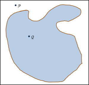
At its heart, this explanation is essentially the classic scenario for Monte Carlo analysis in which the area of an irregular shape (say a lake), $$A_I$$, is estimated by surrounding it with a regular shape (say a square plot of land) of known area, $$A_R$$.

Monte Carlo Lake

The point $${\mathcal P}$$, which falls within $$A_R$$ but outside $$A_I$$ is termed a ‘miss’. The point $${\mathcal Q}$$, which falls within $$A_I$$ is termed a ‘hit’. By distributing points uniformly within $$A_R$$ and counting the ratio of hits, $$N_h$$, to total points used, $$N$$, the area of the irregular shape can be estimated as

\[ \frac{A_I}{A_R} = \frac{N_h}{N} \; ,\]

where the estimate becomes exact as $$N$$ tends to infinity.

The only difference with the classic Monte Carlo problem and the thin foil problem is that the irregular shape in the foil scenario is built out of many non-contiguous pieces.

Halliday and Resnick then generalize this definition by separating the universe of outcomes into more than two choices – hit or miss. They basically subdivide the hit space into additional outcomes like ‘hit the plate and break it into 3 pieces’ or ‘hit the plate and break it into 5 pieces’, and so on. Each of these outcomes can have their respective scattering cross sections given by

\[ \sigma_3 = \frac{A}{N} \frac{I_3}{I_0} \]

for the former case and

\[ \sigma_5 = \frac{A}{N} \frac{I_5}{I_0} \]

for the latter.  Note that the factor $$\frac{A}{N}$$ lends units of area to the cross section, but otherwise just comes along for the ride.

An additional generalization to nuclear and particle physics occurs when the universe of possibilities is expanded to account number of particles scattered into a particular direction or to distinguish encounter when the species changes.

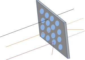
For scattering direction, the scenario looks something like

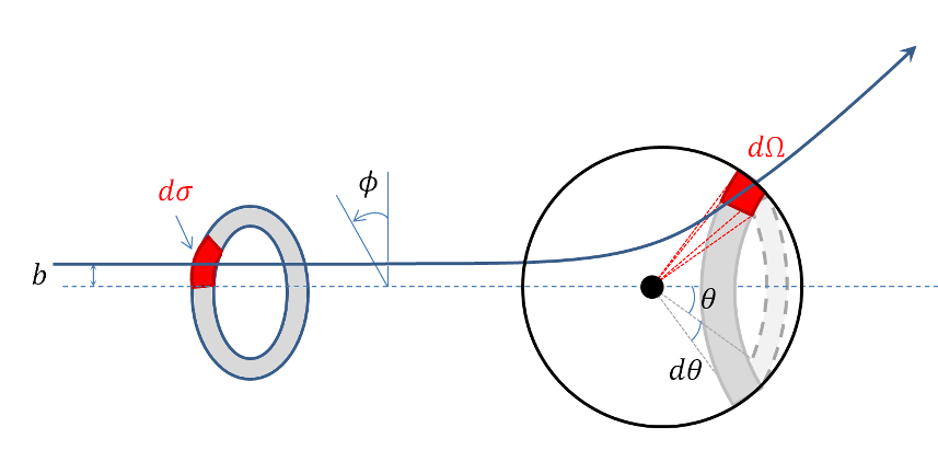
Scattering

where the black trajectory is not scattered, the orange by a little, and the maroon by a lot.

For the case where the species changes, there can be dramatic differences like those listed in Modern Physics by Kenneth Krane. He asks the reader to consider the cross section for the following reactions involving certain isotopes of iodine and xenon:

\[ \begin{array}{lr} I + n \rightarrow I + n & \sigma = 4 b \\ Xe + n \rightarrow Xe + n & \sigma = 4 b \\ I + n \rightarrow I + \gamma & \sigma = 7 b\\ Xe + n \rightarrow Xe + \gamma & \sigma = 10^6 b \end{array} \; . \]

The first two reactions are inelastic scattering, the last two are neutron capture, and the units on cross section are in barns $$b= 10^{-28} m^2$$.

Now I appreciate that nuclear physicists like to work from the thin foil picture, and that, as a result, the definitions of cross section inherit the units from the geometric factor $$A/N$$ out in front. But in reality, their thinking isn’t really consistent with that. In the iodine and xenon example, the absolute values of cross sections are unimportant. What matters is that the likelihood that iodine and xenon will inelastically scatter a neutron are the same while the likelihood of these two elements capturing a neutron are 5 orders of magnitude different, with xenon a 100,000-times more likely.

So why bother assigning cross sections units of area. More physics would be unified if traditional cross sections derived in the above fashion were consistently reinterpreted to be Monte Carlo ratios. This improvement in thinking would unite classical and quantum concepts and would accommodate both deterministic and stochastic systems (regardless of the origin of the randomness). It would also remove that pedagogical thorn of the total scattering cross section of the $$1/r$$ potential as being infinite (which is hard to swallow and makes the cross section seem dodgy when learning it). The question simply no longer holds any meaning. The new interpretation would be that the ratio of particles scattered in any fashion relative to the number sent into the $$1/r$$ scatterer is exactly $$1$$ – i.e. every particle scatters a little. That is the essence of the ‘explanation’ of the infinite cross section (even in classical physics). There would be no area and thus no infinite area as well. It would also put $$1d$$ scattering off of step potentials on the same footing as $$3d$$ scattering. The transmission and reflection coefficients $$T$$ and $$R$$ now would have the same meaning as the scattering cross section. No superfilous and distracting units would separate one from the other.

Unfortunately, I doubt that the physics community would ever actually give up on nearly a century of data, but one can dream.

Vectors and Forms: Part 4 – Vector Identities II

In this final installment on Schleifer’s approach to differential forms and their application to vector calculus, I thought I would take a look at two inter-related items with which Schleifer seems to have had problems. Both of these items deal with using the primitive correspondences to abstractly derive new relations. Before proceeding, it is important to point out that he generally avoids identities involving second derivatives except for the trivial $$\nabla \times (\nabla \phi) = 0$$ and $$\nabla \cdot (\nabla \vec A) = 0$$. As a result, he missed a very interesting opportunity to drive home an important distinction between functions and vectors/forms. As an example of this distinction, reconsider the curl-of-the-curl derived last week.

In vector calculus notation, the curl-of-the-curl identity can be rearranged to give a definition of the Laplacian of a vector

\[\nabla^2 \vec A = \nabla ( \nabla \cdot \vec A) – \nabla \times (\nabla \times \vec A) \; .\]

From the primitive correspondences, the divergence is given by

\[ \nabla \cdot \vec A \Leftrightarrow * d * \phi_A \]

and the curl by

\[ \nabla \times (\nabla \times \vec A) \Leftrightarrow * d \phi_A \; .\]

So the curl-of-the-curl identity can be used to define the differential forms expression for the Laplacian of a vector as given by the correspondence

\[ \nabla^2 \vec A \Leftrightarrow (d * d * – * d * d) \phi_A \; .\]

The natural follow-on question to ask is if this definition is consistent with the expressions for the scalar Laplacian

\[ \nabla^2 f = ( \partial_x^2 + \partial_y^2 + \partial_z^2 ) f \]

introduced in more elementary applications.

Based on the primitive correspondences, the scalar Laplacian naively translates to

\[ \nabla ^2 f \Leftrightarrow * d * d \, f \; \]

So what’s up? Why are they different. Well we can partially fix the difference by subtracting (or adding) a term with the operator $$ d * d * $$ acting on $$f$$ since

\[ d * f = d (f dx \wedge dy \wedge dz ) = 0 \; ,\]

since there is no way for the exterior derivative to raise a 3-form to a higher rank in 3 dimensions, regardless of the functional form of $$f$$.

So we can express the scalar Laplacian as

\[ \nabla^2 f \Leftrightarrow (- d * d * + * d * d) f \; \]

compared to the vector Laplacian

\[ \nabla^2 \vec A \Leftrightarrow (d * d * – * d * d) \phi_A \; .\]

Okay their form is now similar, but why the difference in sign? Well, the sign difference is accepted in the mathematical community and is a consequence of the rank of the form.

The Laplacian of an arbitrary form has the general formula

\[ \nabla ^2 \Leftrightarrow \delta d + d \delta \; ,\]

where the operator

\[ \delta = (-1)^{(np+n+1)} * d * d \; ,\]

where $$n$$ is the dimension of the space, and $$p$$ is the rank of the differential form. If $$n$$ is even then $$\delta = – * d *$$ and if $$n$$ is odd $$\delta = (-1)^p * d * $$. Thus in three dimensions, a $$0$$-form (scalar) has a Laplacian of a different form than a $$1$$-form. We ‘discovered’ this distinction by abstractly manipulating the primitive correspondences (even though Schleifer doesn’t); however, we have found a quantity where the sign differs between the first and the last term. It isn’t clear how this arose or whether it is correct or an artifact of Schleifer’s instance to map vectors and forms so closely. Since he avoids the second derivative identities, we’ll never know what his view on this is.

A related point is the endnote in which Schleifer states that the only type of vector identity he was unable to prove were ones of the form

\[ \nabla \times (\vec A \times \vec B) = (\vec B \cdot) \vec A + \Leftrightarrow *d(*(\phi_A \wedge \phi_B)) \; . \]

Now this statement is a bit of a mystery to me. The cross product has the established mapping

\[ \nabla \times (\vec A \times \vec B) \Leftrightarrow *d(*(\phi_A \wedge \phi_B)) \; ,\]

which expands to

\[ * (\phi_A \wedge \phi_B) = (A_y B_z – A_z B_y) dx \\ + (A_z B_x – A_x B_z) dy \\ + (A_x B_y – A_y B_x) dz \; .\]

For notational convenience define

\[ C_x = A_y B_z – A_z B_y \; , \]
\[ C_y = A_z B_x – A_x B_z \; , \]
and
\[ C_Z = A_x B_y – A_y B_x \; .\]

These three equations can be compactly written as

\[ C_i = \epsilon_{ijk} A_j B_k \]

The curl of this cross-product translates to the language of differential forms as

\[ d * (\phi_A \wedge \phi_B) = C_{x,y} dy \wedge dx + C_{x,z} dz \wedge dx + C_{y,x} dx \wedge dy \\ + C_{y,z} dz \wedge dy + C_{z,x} dx \wedge dz + C_{z,y} dy \wedge dz \; .\]

The pattern exhibited by the coefficients of the two-forms also leads to a compact expression

\[ d * (\phi_A \wedge \phi_B) = \epsilon_{k \ell m} \partial_{\ell} C_k dx^m \; \]

Combining these last two expressions yields precisely what one gets from the classical vector manipulation

\[ \nabla \times (\vec A \times \vec B) = \epsilon_{ijk} \partial_j [\vec A \times \vec B]_k = \epsilon_{ijk} \partial_j \epsilon_{k \ell m} A_\ell B_m \]

which, up to a trivial change of indices, is the same. So why Schleifer says he can’t prove it I don’t know. Perhaps he is trying to say is that in the identity

\[ \nabla \times (\vec A \times \vec B) = (\vec B \cdot \nabla) \vec A – (\vec A \cdot \nabla) \vec B + (\nabla \cdot \vec B) \vec A – (\nabla \cdot \vec A) \vec B \]

there is no proper differential forms mapping of $$(\vec B \cdot \nabla) \vec A$$. Let me say that it even if it doesn’t, it really isn’t a concern. It is not like he actually exploits the abstract language to derive new expressions using the primitive correspondences. If he did he would have discovered the switching sign on the Laplacian.

Overall, I admire Schleifer’s goal but I am concerned about two aspects of this particular program. First is the notational complexity that comes about. For example, $$\vec A \cdot \vec B \Leftrightarrow *(\phi_A \wedge * \phi_B)$$ The need to wrap the expression with parentheses to distinguish $$*\phi_A \wedge * \phi_B \neq *(\phi_A \wedge *\phi_B)$$ makes the notation clunky. Second, and more important, it seems that the desire to continuously re-express the language of differential forms back to vector calculus undercuts the pedagogy and, as shown with the Laplacian, leads to more questions than answers. Hopefully with more time this program can be rescued but for now it doesn’t quite seem ready for prime time.

Vectors and Forms: Part 3 – Vector Identities I

The last column introduced the exterior derivative operator $$d$$ and, using this operator and the language of differential forms, developed analogous expressions for the classical vector concepts of gradient, divergence, and curl, each being given by

\[ \nabla f \Leftrightarrow d f \; ,\]

\[ \nabla \cdot \vec A \Leftrightarrow *d* \phi_A \; , \]

and

\[ \nabla \times \vec A \Leftrightarrow * d \phi_A \; , \]

respectively. These relations, collectively, assume the name of the primitive correspondences.

This installment tackles the extension of these ideas to the classical set ‘vector derivative identities’ that tend to crop up whenever vector calculus is employed (usually in electrodynamics or fluid mechanics) and which are often unclear or unmotivated. One of the main thrusts behind the work of Schleifer to publish the correspondences between vector calculus and the language of differential forms was the hope that a deeper understanding of the underlying, unified structure would become apparent. It was this aim that originally attracted my attention to his paper.

The first set of identities to be discussed are the curl of the gradient is zero,

\[ \nabla \times \nabla f = 0 \; , \]

and the divergence of a curl is zero,

\[ \nabla \cdot \nabla \times \vec A = 0 \; .\]

From the point-of-view of vector calculus, these two identities, while looking similar, don’t flow from any common source. But each of these is an expression of the much simpler identity $$d^2 = 0$$. Indeed, it was the desire to unite these dispparate relations that led, in great part, to the invention of the language of differential forms.

To prove that the curl of a gradient is zero explicitly use the first and third primitive correspondences

\[ \nabla \times (\nabla f) \Leftrightarrow *d(d f) = * d^2 f = 0 \; .\]

Likewise, the demonstration that the curl of a vector field is divergence-free involves the second and the third of the primitive correspondences
\[ \nabla \cdot \nabla \times \vec A \Leftrightarrow (*d*)(*d\phi_A) = * d ** d \phi_A = * d^2 \phi_A = 0 \; .\]

Most of the more exotic vector identities require a bit more work to demonstrate them explicitly and are not done with abstract manipulation but, instead, with coordinates. This is not especially concerning, since the aim here is to bridge the gap between the two approaches and not to demonstrate internal consistency or proficiency in either one.

Curl-of-the-curl

One such vector identity is the curl-of-the-curl, $$\nabla \times (\nabla \times \vec A)$$, which arises often in the study of Maxwell’s equations. The traditional way to perform the identity is by index-gymnastics involving the Levi-Cevita tensor density and the Kronecker delta. Appling this technology yields

\[\nabla \times (\nabla \times \vec A) = \epsilon_{ijk} \partial_j ( \epsilon_{k \ell m} \partial_\ell A_m ) = (\delta_{i\ell}\delta_{jm} – \delta_{im}\delta_{j\ell} ) \partial_j \partial_\ell A_m \; .\]

Resolving the Kronecker deltas yields the index equation

\[\nabla \times (\nabla \times \vec A) = \partial_j \partial_i A_j – \partial_j \partial_j A_i \; ,\]

which has the immediate translation into ‘vector language’ of

\[ \nabla \times (\nabla \times \vec A) = \nabla (\nabla \cdot \vec A) – \nabla^2 \vec A \;. \]

The differential forms way is to start with the standard correspondence

\[\phi_A = A_x dx + A_y dy + A_z dz \]

and then to apply the third primitive correspondence

\[ *d \phi_A = (A_{z,y} – A_{y,z}) dx + (A_{x,z} – A_{z,x}) dy + (A_{y,x} – A_{x,y}) dz \; . \]

Applying the exterior derivative an additional time and accounting for the properties of the wedge product yields the two-form

\[ d*d \phi_A =( A_{x,zx} – A_{z,xx} – A_{z,yy} + A_{y,zy} ) dx \wedge dy \\ + ( A_{y,xy} – A_{x,yy} – A_{x,zz} + A_{z,xz} ) dy \wedge dz \\ + ( A_{z,yz} – A_{y,zz} – A_{y,xx} + A_{x,yx} ) dz \wedge dx \; .\]

Applying the Hodge star operator to get the dual gives

\[ *d*d \phi_A = (\partial_j \partial_i A_j – \partial_j \partial_j A_i) dq^i \; ,\]

where $$dq^i = dx, dy, dz$$ for $$ i = i, 2, 3$$.

Employing the vector-to-form correspondence, one sees that these are the same components as in the vector form, once the common, self-cancelling terms associated with $$i=j$$ are taken into account.

Gradient-of-the-dot

The next identity is the gradient of a dot-product. Based on the primitive correspondences, one can start with

\[ \nabla (\vec A \cdot \vec B) \Leftrightarrow d(*(\phi_A \wedge *\phi_B)) \; .\]

To see how this comes out, begin with the recognition that the dot-product is a scalar function so that it is particularly easy to move between vectors and forms. The form-equivalent of the gradient of this scalar function is

\[ d (A_x B_x + A_y B_y + A_z B_z) = \partial_i (A_x B_x + A_y B_y + A_z B_z ) dq^i \; ,\]

where $$dq^i$$ is as defined above.

What remains is to expand the action of the partial derivative and show that the result forms translate into the desired vector identity.

\[ \partial_i (A_j B_j) = (A_{x,i} B_x + A_{y,i} B_y + A_{z,i} B_z) + ( A_x B_{x,i} + A_y B_{y,i} + A_z B_{z,i} ) \; .\]

For simplicity, focus on the $$i=x$$ and strategically add and subtract two groups of terms
\[ A_{x,x} B_x + A_{y,x} B_y + A_{z,x} B_z \\ + (A_{x,y} B_y – A_{x,y} B_y) + (A_{x,z} B_z – A_{x,z} B_z) + B \leftrightarrow A \; .\]

Next group the terms into the suggestive form

\[ B_x A_{x,x} + B_y A_{x,y} + B_z A_{x,z} \\ + B_y (A_{y,x} – A_{x,y}) + B_z(A_{z,x} – A_{x,z} ) + B \leftrightarrow A \; .\]

The next step requires a peek back into the language of vectors. Since the curl is given by

\[ \nabla \times \vec A = (A_{z,y} – A_{y,z} ) \hat e_x + (A_{z,y} – A_{y,z} ) \hat e_y + (A_{z,y} – A_{y,z} ) \hat e_x \; ,\]

the re-arranged term can be re-written as

\[ B_x A_{x,x} + B_y A_{x,y} + B_z A_{x,z} + B_y (A_{y,x} – A_{x,y}) + B_z(A_{z,x} – A_{x,z} ) \\ + B \leftrightarrow A = (\vec B \cdot \nabla) A_x + B_y [\nabla \times \vec A]_z – B_z [\nabla \times \vec A]_y + B \leftrightarrow A\; .\]

The final two terms on the right can be further re-written as

\[ B_x A_{x,x} + B_y A_{x,y} + B_z A_{x,z} + B_y (A_{y,x} – A_{x,y}) + B_z(A_{z,x} – A_{x,z} ) \\ + B \leftrightarrow A = (\vec B \cdot \nabla) A_x + [\vec B \times (\nabla \times \vec A) ]_x + B \leftrightarrow A \; .\]

And so we arrive at the final vector calculus identity for the gradient of the dot-product, without a really meaningful differential form analog.

\[ \nabla ( \vec A \cdot \vec B ) = (\vec B \cdot \nabla) \vec A + \vec B \times (\nabla \times \vec A) + (\vec A \cdot \nabla) \vec B + \vec A \times (\nabla \times \vec B) \]

This was to be expected since the motivation for the addition and subtraction of those additional terms was only to manipulate the partial derivative expression into something familiar from the vector calculus.

Divergence of a cross

The final identity to be explored in this column is the divergence of a cross. In vector calculus, the divergence of a cross expands to

\[ \nabla \cdot (\vec A \times \vec B) = (\nabla \times \vec A) \cdot \vec B – (\nabla \times \vec B) \cdot \vec A \]

Using the second and third primitive correspondences, the proposed analog in the language of differential forms is

\[ \nabla \cdot (\vec A \times \vec B) \Leftrightarrow *d*( *(\phi_A \wedge \phi_B) ) \; .\]

Tackling the right-hand side is easier by ommitting the leading Hodge star operator to give

\[ d*( *(\phi_A \wedge \phi_B) ) = d\left[ (A_y B_z – A_z B_y) dy \wedge dz \\ + (A_z B_x – A_x B_z) dz \wedge dx + (A_x B_y – A_y B_x) dx \wedge dy \right] \; .\]

Re-applying this operator yields

\[ *d*( *(\phi_A \wedge \phi_B) ) = (A_{y,x} B_z – A_{z,x} B_y ) + (A_{z,y} B_x – A_{x,y} B_z ) \\ + ( A_{x,z} B_y – A_{y,z} B_x ) – B \leftrightarrow A \; .\]

Grouping terms suggestively gives
\[ *d*( *(\phi_A \wedge \phi_B) ) = (A_{z,y} – A_{y,z}) B_x + (A_{x,z} – A_{z,x}) B_y \\ + (A_{y,x} – A_{x,y}) B_z – B \leftrightarrow A \; ,\]

from which it is obvious that

\[ *d*( *(\phi_A \wedge \phi_B) ) = (\nabla \times \vec A) \cdot \vec B – (\nabla \times \vec B) \cdot \vec A \; .\]

Next week, I’ll close out this subject with a look at the equivalent operator to the Laplacian and with a comment on the identities that Schleifer claims he couldn’t prove.

Vectors and Forms: Part 2 – Div and Curl

In order to extend the results from last week into the realm of classical vector analysis, we must introduce an additional operator called the exterior derivative and which is denoted by $$d$$. The exterior derivative can be thought of as the classical nabla $$\vec \nabla$$ on steroids since it is a bit more versatile and works in spaces of arbitrary dimension.

The defining property of the exterior derivative is that when it operates on a differential form $$\phi(x,y,z)$$ it produces a new differential form $$d\phi$$ of one higher order. So if $$\phi$$ is an $$n$$-form then $$d\phi$$ is an $$n+1$$-form. To understand how this operation is carried out, we start with its action on a function (i.e. a $$0$$-form). In this case

\[ df = \frac{\partial f}{\partial x} dx + \frac{\partial f}{\partial y} dy + \frac{\partial f}{\partial z} dz \; ,\]

which is just what is expected from basic calculus. The remaining piece of the definition is to see what the action of $$d$$ is on a $$1$$-form. Since it results in a $$2$$-form, we can suspect that may involve the wedge product and we would be right. Specifically, suppose that the one form is given by

\[ \phi = A_x dx \]

then

\[ d \phi = d (A_x dx) = \frac{\partial A_x}{\partial x} dx \wedge dx + \frac{\partial A_y}{\partial y} dy \wedge dx + \frac{\partial A_z}{\partial z} dz \wedge dx \; .\]

From the anti-symmetry property of the wedge product, this result simplifies to

\[ d \phi = \frac{\partial A_y}{\partial y} dy \wedge dx + \frac{\partial A_z}{\partial z} dz \wedge dx \; .\]

The generalization to more complex $$1$$-forms is obvious.

As a result of these properties, the exterior derivative satisfies $$d^2 = dd = 0$$ regardless of what it operates on.

We are now in the position to adapt the language of differential forms to some familiar results of vector calculus.

The core adaptations are for the divergence and curl. The remaining vector calculus identities more or less flow from these.

The expression for the divergence start with the expression for the corresponding one form

\[ \phi_A = A_x dx + A_y dy + A_z dz \; . \]

Apply the Hodge star operator first

\[ *\phi_A = A_x dy \wedge dz + A_y dz \wedge dx + A_z dx \wedge dy \; .\]

The application of the exterior derivative only produces derivatives for the excluded variable in the wedge product

\[ d*\phi_A = A_{x,x} dx \wedge dy \wedge dz + A_{y,y} dy \wedge dz \wedge dx + A_{z,z} dz \wedge dx \wedge dy \; , \]

where the term

\[ A_{x,x} = \frac{\partial A_x}{\partial x} \]

and so on for the other terms.

All of the wedge products are cyclic permutations of $$dx \wedge dy \wedge dz$$ so rearrangement involves no changes of sign. A further application of the Hodge star operator give the zero form

\[ *d*\phi_A = A_{x,x} + A_{y,y} + A_{z,z} \Leftrightarrow \vec \nabla \cdot \vec A \; .\]

The curl, which is handled in a similar way, is expressed as

\[ \vec \nabla \times \vec A \Leftrightarrow *d\phi_A \; .\]

The proof is reasonably easy. Start again with the expression for the corresponding form

\[ \phi_A = A_x dx + A_y dy + A_z dz \; \]

and then operate on it with the exterior derivative to get

\[ d \phi_A = A_{x,y} dy \wedge dx + A_{x,z} dz \wedge dx + A_{y,x} dx \wedge dy \\ + A_{y,z} dz \wedge dy + A_{z,x} dx \wedge dz + A_{z,y} dy \wedge dz \; \]

Organizing the terms in lexicographical order (i.e. $$dx \wedge dy$$, $$dx \wedge dz$$, and $$dy \wedge dz$$), accounting for changes in sign as terms are swapped, gives

\[ d\phi_A = (A_{y,x}-A_{x,y}) dx \wedge dy \\ + (A_{z,y}-A_{y,z}) dy \wedge dz \\ + (A_{x,z}-A_{z,x}) dz \wedge dx \; \]

The final step is to apply the Hodge star operator to arrive at

\[ *d\phi_A = (A_{y,x}-A_{x,y}) dz + (A_{z,y}-A_{y,z}) dx + (A_{x,z}-A_{z,x}) dy \; , \]

which proves the correspondence

\[ *d\phi_A \Leftrightarrow \vec \nabla \times \vec A \; .\]

Next column, I’ll expand on the algebra of differential forms just a bit and then will apply the results introduced here to prove a host of vector calculus identities.

Vectors and Forms: Part 1 – The Basics

I thought it might be nice to have a change of pace in this column and discuss some differential geometry and the relationship between classical vector analysis and the calculus of differential forms. In large measure, this dabbling is inspired by the article Differential forms as a basis for vector analysis – with applications to electrodynamics by Nathan Schleifer which appeared in the American Journal of Physics 51, 1139 (1983).

While I am not going to go into as much detail in this post as Schleifer did in his article, I do want to capture the flavor of what he was trying to do and set the groundwork for following posts on proving some of the many vector identities that he tackles (and perhaps a few that he doesn’t). At the botttom of all these endeavors is the pervading similarity of all of the various integral theorems of vector calculus.

The basis premise of the operation is to put into a one-to-one correspondence a classical vector expressed as

\[ \vec A = A_x \hat e_x + A_y \hat e_y + A_z \hat e_z \]

with an associated differential one-form

\[ \phi_{A} = A_x dx + A_y dy + A_z dz \; .\]

The elements of both descriptions form a vector space; that is to say that the 10 axioms of a vector space are satisfied by the objects in $$\{dx, dy, dz\}$$ just as they are satisfied by $$\{\hat e_x , \hat e_y, \hat e_z\}$$.

If decomposition into components were all that was required, the two notations would offer the same benefits with the only difference being the superficial differences in the glyphs of one set compared to another.

However, we want more out of our sets of objects. Exactly what additional structure each set caries and how it is notationally encoded is the major difference between the two approaches.

Typically, classical vectors are given a metric structure such that

\[ \hat e_i \cdot \hat e_j = \delta_{ij} \]

and a ‘cross’ structure such that

\[ \hat e_i \times \hat e_j = \epsilon_{ijk} e_k \; .\]

Differential one-forms differ in that they are given only the ‘cross’ structure in the form
\[ dy \wedge dz = – dz \wedge dy \; ,\]
\[ dz \wedge dx = – dx \wedge dz \; ,\]
\[ dx \wedge dy = – dy \wedge dx \; ,\]

where the wedge product $$dx \wedge dy$$ is sensibly called a two-form, indicating that it is made up of two one-forms.

Like the vector cross-product, the wedge product anti-commutes, implying that

\[ dx \wedge dx = 0 \; ,\]

with an analogous formula for $$dy$$ and $$dz$$.

Despite these similarities, the wedge product differs in one significant way from its vector cross-product cousin in that it is also associative so that no ambiguity exists by saying

\[ dx \wedge (dy \wedge dz) = (dx \wedge dy) \wedge dz = dx \wedge dy \wedge dz \; .\]

These algebraic rules are meant to sharply distinguish a point that is lost in classical vector analysis – namely that a vector defined in terms of a cross-product (i.e $$\vec C = \vec A \times \vec B$$) is not really a vector of the same type as the two vectors on the right-hand side that define it. That this must be true is easily (if somewhat startlingly) seen by the fact that when we consider the transformation of coordinates, the right-hand side needs two factors (one for $$\vec A$$ and one for $$\vec B$$) while the left-hand side needs only one. From a geometric point-of-view, we are exploiting a natural association between a plane spanned by $$\vec A$$ and $$\vec B$$ and the unique vector (up to a sign) that is perpendicular to it. This later obsservation is fully encoded into the structure of differential forms by defining the Hodge star operator such that

\[ dy \wedge dz \equiv *dx \; ,\]
\[ dz \wedge dx \equiv *dy \; ,\]
\[ dx \wedge dy \equiv *dz \; .\]

Also note that the Hodge star can be toggeled in the sense that

\[ *(dy \wedge dz) = **dx = dx \; ,\]

with similar expressions for the other two combinations.

Since the wedge product is associative, the Hodge star can be extended to operate on a three-form to give

\[ *(dx \wedge dy \wedge dz) = 1 \; , \]

which is interpreted as associating volumes with scalars.

All the tools are in place to follow the program of Schleifer for classical vector analysis. Note: some of these tools need to be modified for either higher dimensional spaces, or for non-positive-definite spaces, or both.

At this point, there may be some worry expressed that since the formalism of differential forms has no imposed metric structure, that we’ve thrown away the dot-product and all its useful properties. That this isn’t a problem can be seen as follows.

The classic dot-product is given by

\[ \vec A \cdot \vec B = A_x B_x + A_y B_y + A_z B_z \; .\]

The equivalent expression, in terms of forms, is

\[ \vec A \cdot \vec B \Leftrightarrow * ( \phi_{A} \wedge *\phi_B )\]

as can be seen as follows:

\[ \phi_B = B_x dx + B_y dy + B_z dz \; , \]

from which we get

\[ *\phi_B = B_x dy \wedge dz + B_y dz \wedge dx + B_z dx \wedge dy \; .\]

Now multiplying, from the left, by $$\phi_A$$ will lead to 9 products, each resulting in a three-form. However, due to the properties of the wedge product, only those products with a single $$dx$$, $$dy$$, and $$dz$$ will survive. These hardy terms are

\[ \phi_A \wedge *\phi_B = A_x B_x dx \wedge dy \wedge dz \\ + A_y B_y dy \wedge dz \wedge dx \\ + A_z B_z dz \wedge dx \wedge dy \; .\]

Accounting for the cyclic permutation of the wedge product this relation can be re-written as

\[ \phi_A \wedge *\phi_B = (A_x B_x + A_y B_y + A_z B_z) dx \wedge dy \wedge dz \; .\]

Applying the Hodge star operator immediately leads to

\[ * (\phi_A \wedge * \phi_B)) = A_x B_x + A_y B_y + A_z B_z \; . \]

In a similar fashion, the cross-product is seen to be
\[ \vec A \times \vec B \Leftrightarrow *(\phi_A \wedge \phi_B) \; .\]

The proof of this follows from

\[ \phi_A \wedge \phi_B = (A_x dx + A_y dy + A_z dz ) \wedge (B_x dx + B_y dy + B_z dz) \; ,\]

which expands to

\[ \phi_A \wedge \phi_B = (A_x B_y – A_y B_x) dx \wedge dy \\ + (A_y B_z – A_z B_y) dy \wedge dz \\ + (A_z B_x – A_x B_z) dz \wedge dx \; .\]

Applying the Hodge star operator gives

\[ *(\phi_A \wedge \phi_B) = (A_x B_y – A_y B_x) dz \\ + (A_y B_z – A_z B_y) dx \\ + (A_z B_x – A_x B_z) dy \equiv \phi_C \; ,\]

which gives an associated vector $$\vec C$$ of

\[ \phi_C \Leftrightarrow \vec C = (A_y B_z – A_z B_y) \hat e_x \\ + (A_z B_x – A_x B_z) \hat e_y \\ + (A_x B_y – A_y B_x) \hat e_z \; .\]

Next week, I’ll extend these results to include the classical vector analysis by use of the exterior derivative.

First-Order Gauss Markov Processes

Change of pace is always good and, in this spirit, this week’s column will aims to model the solutions of the First-order Gauss Markov process. A First-order Gauss Markov process is a stochastic process that is used in certain applications for scheduling the injection of process noise into filtering methods. The basic idea is that during certain time periods, the internal physical process modelled in the filter will be insufficient due to the turning on and off of some additional, unmodelled force. Typical applications include the application of man-made controls to physical systems to force certain desirable behaviors.

The formulation of the First-order Gauss Markov process is usually done in terms of a stochastic equation. For simplicity, the scalar form will be studied. The generalization to the case with many components is straightforward and nothing is gained by the notational clutter. The equation we will analyze is
\[ {\dot x} = -\frac{1}{\tau} x + w \quad ,\]
where $$x(t)$$ is defined as the state and $$w$$ is a inhomogeneous noise term. In the absence of the noise, the solution is given by a trivial time integration to yield
\[ x_{h}(t) = x_{0} e^{ -(t-t_{0})/\tau } \quad , \]
assuming that $$x(t=t_{0}) = x_{0}$$. The solution $$x_h(t)$$ is known as the homogeneous solution and, as has often been discussed in this column, it will help in integrating the inhomogeneous term $$w$$. Ignore, for the moment, that $$w$$ (and, as a result, $$x$$) is a random variable. Treated as just an ordinary function, $$w$$ is a driving term that can be handled via the state transition matrix (essentially a one-sided Green’s function for an initial-value problem). Recall that a state transition matrix (STM) is defined as the object linking the state at time $$t_{0}$$ to the state at time $$t$$ according to
\[ x(t) = \Phi(t,t_{0}) x(t_{0}) \quad , \]
thus, by the definition, the STM is obtained as
\[ \Phi(t,t_{0}) = \frac{\partial x(t)}{\partial x(t_{0})} \quad . \]
Taking the partial derivative of homogeneous solution as required by the definition of the STM gives
\[ \Phi(t,t_{0}) = e^{ -(t-t_{0})/\tau } \quad . \]
The solution of the inhomogeneous equation is then given as
\[ x(t) = x_{h}(t) + \int_{t_{0}}^{t} \Phi(t,t’) w(t’) dt’ \quad .\]
As a check, take the time derivative of this expression to get
\[ {\dot x}(t) = {\dot x}_{h}(t) + \frac{d}{dt} \left[ \int_{t_{0}}^{t} \Phi(t,t’) w(t’) dt’ \right] \; \]
and then eliminate the time derivative on the two terms on the right-hand side by using the homogeneous differential equation for the first term and by using the Liebniz rule on the second term involving the integral
\[ {\dot x}(t) = -\frac{1}{\tau} x_{h}(t) + \Phi(t,t) w(t) + \int_{t_{0}}^{t} \frac{\partial \Phi(t,t’)}{\partial t} w(t’) dt’ \quad . \]
Since the following two conditions
\[ \Phi(t,t) = 1 \quad , \]
and
\[ \frac{\partial \Phi(t,t’)}{\partial t} = -\frac{1}{\tau} \Phi(t,t’) \quad , \]
are met, they can be substituted into the above expression. Doing so yields
\[ {\dot x}(t) = -\frac{1}{\tau} x_{h}(t) + w(t) – \frac{1}{\tau} \int_{t_{0}}^{t} \Phi(t,t’) w(t’) dt’ \; .\]
Grouping the terms in a suggestive way gives
\[ {\dot x}(t) = -\frac{1}{\tau} \left[ x_{h}(t) + \int_{t_{0}}^{t} \Phi(t,t’) w(t’) dt’ \right] + w(t) \; \]
from which immediately springs the recognition that
\[ {\dot x}(t) = -\frac{1}{\tau} x(t) + w(t) \quad \; , \]
which is what we were trying to prove.

It is worth noting that the condition listed for the time derivative of the STM is a specific example of the familiar form
\[ \frac{\partial \Phi(t,t’)}{\partial t} = A(t) \Phi(t,t’) \quad ,\]
where $$A(t)$$, known sometimes as the process matrix, is generally given by
\[ A(t) = \frac{\partial {\mathbf f}( {\mathbf x} (t) ) }{\partial {\mathbf x}(t)} \; .\]

With the general formalism well understood, the next step is to generate solutions. Since $$w(t)$$ is a noise term, each ensemble of realizations will birth a different response in $$x(t)$$ via the driving term in
\[ x(t) = x_{0} e^{ -(t-t_{0})/\tau } + \int_{t_{0}}^{t} e^{ -(t-t’)/\tau } w(t’) dt’ \; .\]
So there are an infinite number of solution and there is no practical way to deal with them as a group but statistically some meaningful statements can be made. The most useful statistical characterizations are found by computing the statistical moments about the origin (i.e. $$E[x^n(t)]$$, where $$E[\cdot]$$ denotes the expectation value of the argument).

In order to do this, we need to say something about the statistical distribution of the noise. We will assume that $$w(t)$$ is a Gaussian white-noise source with zero mean, a variance of $$q$$, and is uncorrelated. Mathematically these assertations amount to the condition $$E[w(t)] \equiv {\bar w} = 0$$ and the condition
\[ E[(w(t)-{\bar w}) (w(s) – {\bar w}) ] = E[ w(t)w(s) – {\bar w} w(t) – {\bar w} w(s) – {\bar w}^2 ] \\ = E[ w(t)w(s) ] = q \delta(t-s) \quad . \]

In addition, we assume that the state and the noise are statistically independent at different times
\[ E[x(t) w(s) ] = E[x(t)] E[w(s)] = 0 \quad . \]
Now we can compute the statistical moments of $$x(t)$$ about the origin.

The first moment is given by
\[ E[x(t)] = E \left[ x_{0} e^{ -(t-t_{0})/\tau } + \int_{t_{0}}^{t} e^{ -(t-t’)/\tau } w(t’) dt’ \right] \; .\]
Since the expectation operator is linear and since it only operates on $$x(t)$$ and $$w(t)$$ (they are the only two random variable) this expression becomes
\[ E[x(t)] = E \left[ x_{0} \right] e^{ -(t-t_{0})/\tau } + \int_{t_{0}}^{t} e^{ -(t-t’)/\tau } E \left[ w(t’) \right] dt’ \; .\]
From its statistical properties, $$E[w(t)] = $$ and so the above expression simplifies to
\[ E[x(t)] = E \left[ x_{0} \right] e^{ -(t-t_{0})/\tau } \; .\]

The second moment is more involved, although no more conceptually complicated, and is given by


\[ E[ x(t)^2 ] = E \left[ x_{0}^2 e^{ -2(t-t_{0})/\tau } \\ + 2 x_{0} e^{ -(t-t_{0})/\tau } \int_{t_{0}}^{t} e^{ -(t-t’)/\tau } w(t’) dt’ \\ + \int_{t_{0}}^{t} e^{ -(t-t’)/\tau } w(t’) dt’ \int_{t_{0}}^{t} e^{ -(t-t”)/\tau } w(t^{\prime\prime}) dt^{\prime\prime} \right] \; \]

Again using the facts that the expectation operator is linear and that the noise is zero mean, the second moment becomes

\[ E[x(t)] = E \left[x_{0}^2\right]e^{ -2(t-t_{0})/\tau } \\ + \int_{t_{0}}^{t} \int_{t_{0}}^{t} e^{ -(2t-t’-t”)/\tau } E \left[ w(t’) w(t^{\prime\prime}) \right] dt’ dt^{\prime\prime} \; .\]

Next we use the fact that the noise auto-correlation resolves to a delta function leaving behind

\[ E[x(t)] = E \left[x_{0}^2\right]e^{ -2(t-t_{0})/\tau } + \int_{t_{0}}^{t} \int_{t_{0}}^{t} e^{ -(2t-t’-t”)/\tau } + q \delta(t’-t”) dt’ dt^{\prime\prime} \; .\]

From there the final step is to use the properties of the delta-function to gid rid of one the integrals and then to explicitly evaluate the remaining one to get

\[ E[x(t)] = E \left[x_{0}^2\right]e^{ -2(t-t_{0})/\tau } + \frac{q \tau}{2} \left( 1 – e^{ -2(t-t_{0})/\tau } \right) \;.\]

With the first two moments in hand it is easy to get the variance

\[ E \left[x^2\right] – E\left[x\right]^2 = \left( E\left[x_{0}^2\right] – E \left[x_{0}\right]^2 \right) e^{-2(t-t_{0})/\tau} + \frac{q\tau}{2} \left(1- e^{-2(t-t_{0})/\tau} \right) \; ,\]

which can be re-written as

\[ {\mathcal P}(t) = {\mathcal P}_0 e^{ -2(t-t_0)/\tau } + \frac{q\tau}{2}\left(1-e^{-2(t-t_{0})/\tau}\right) \quad , \]

where $${\mathcal P_0} = \left( E\left[x_0^2\right] – E\left[x_0\right]^2 \right)$$ is the initial covariance.

The final step is to discuss exactly what these equations are telling. The solution for the mean suggests that the mean will, after a long time, settle in at a value of zero regardless of the initial conditions for $$x_0$$. The variance equation then tells us that the uncertainty or dispersion about this zero-mean grows as $$\sqrt{t}$$ (since the only long-time term in the variance is proportional to $$t$$). This behavior is suggestive of a random walk. One of the more useful applications of this formalism to schedule in the parameter $$q$$ and being non-zero only within a certain time span. During this time span, the variance of process ‘opens up’ thereby allowing more freedom for a filter to heed measurement data rather than paying strict attention to its internal process. Thus a First-order Gauss Markov process, when scheduled into an underlying physical process, allows for modern filters to tracking unmodeled forces.

More Matrices, Rows, and Columns

Last week I covered some nice properties associated with the looking at a matrix in terms of its rows and its columns as entities in their own sense. This week, I thought would put some finishing touches on these points with a few additional items to clean up the corners, as it were.

Transforming Coordinates

The biggest reason, or perhaps clue, for regarding row and/or columns of matrices as having an identity apart from the matrix itself comes from the general theory of changing coordinates. We start in two dimensions (the generalization to $$N$$ dimensions is obvious) with an arbitrary vector $$\vec A$$ and two different coordinate systems $${\mathcal O}$$ and $${\mathcal O}’$$ being used in its description. The relevant geometry is shown below.

coordinate_transformation

We can consider the two frames as being spanned by the set of orthogonal vectors $$\{\hat e_x, \hat e_y\}$$ and $$\{\hat e_{x’}, \hat e_{y’}\}$$, respectively. Now the obvious decomposition of the vector is both frames leads to

\[ \vec A = A_x \hat e_x + A_y \hat e_y \]

and

\[ \vec A = A_{x’} \hat e_{x’} + A_{y’} \hat e_{y’} \; .\]

The fun begins when we note that the individual components of $$\vec A$$ are obtained by taking the appropriate dot-products between it and the basis vectors. It is straightforward to see that

\[ A_x = \vec A \cdot \hat e_x \]

since

\[ \vec A \cdot \hat e_x = \left(A_x \hat e_x + A_y \hat e_y \right) \cdot \hat e_x = A_x \hat e_x \cdot \hat e_x + A_y \hat e_y \cdot \hat e_x = A_x \; .\]

The last relation follows from the mutual orthogonality of the basis vectors, which is summarized as

\[ \hat e_i \cdot \hat e_j = \delta_{ij} \; ,\]

where $$\delta_{ij}$$ is the usual Kronecker delta.

The fun builds when we allow $$\vec A$$ to be expressed in the alternate frame from the one whose basis vector is being used in the dot-product. This ‘mixed’ dot-product serves as the bridge needed to cross between the two frames as follows.

\[ \vec A \cdot \hat e_x = \left( A_{x’} \hat e_{x’} + A_{y’} \hat e_{y’} \right) \cdot \hat e_x \; .\]

On one hand, $$\vec A \cdot \hat e_x = A_x$$, as was established above. On the other, it takes the form

\[\vec A \cdot \hat e_{x’} = A_{x’} \hat e_{x’} \cdot \hat e_{x} + A_{y’} \hat e_{y’} \cdot \hat e_{x} \; .\]

Equating the two expressions gives the ‘bridge relation’ between the two frames. Carrying this out for the other components leads to the matrix relation between the components in different frames given by

\[ \left[ \begin{array}{c} A_{x’} \\ A_{y’} \end{array} \right] = \left[ \begin{array}{cc}\hat e_{x’} \cdot \hat e_{x} & \hat e_{x’} \cdot \hat e_y \\ \hat e_{y’} \cdot \hat e_{x} & \hat e_{y’} \cdot \hat e_y \end{array} \right] \left[ \begin{array}{c} A_x \\ A_y \end{array} \right] \; .\]

A bit of reflection should allow on to see that the rows of the $$2 \times 2$$ matrix that connects the right-hand side to the left are the components of $$\hat e_{x’}$$ and $$\hat e_{y’}$$ expressed in the $${\mathcal O}$$ frame. Likewise, the columns of the same matrix are the components of $$\hat e_x$$ and $$\hat e_y$$ expressed in the $${\mathcal O}’$$ frame. Since there is nothing special about which frame is really labelled $${\mathcal O}$$ and which is labelled $${\mathcal O}’$$, it follows logically that the transpose of the matrix must be its own inverse. Therefore, we’ve arrived at the concept of an orthogonal matrix.

Units

Following hard on the heels of the previous result is a comment on the units born by the elements of a matrix. While mathematics likes to have pure numbers, the practicing physical scientist is not afforded that luxury. If we regard an arbitrary matrix has having units (that is each element has the same units) then the column arrays $$|e_i\rangle$$ must also have the same units. But the row arrays $$\langle \omega_j|$$ must have the inverse units for two very good reasons.

First the relations $$\langle \omega_j | e_i \rangle = \delta_{ij}$$ and the $$\sum_i |e_i\rangle \langle \omega_i| = {\mathbf Id}$$ (where $${\mathbf Id}$$ is the $$N \times N$$ identity matrix) demand that the rows have inverse units compared to the columns. Second, the determinant of the original matrix has units of the original base raised to the $$N$$-th power for a $$N \times N$$ matrix. Classical matrix inverse theory requires that the components of the inverse are proportional to the determinant of some $$N-1 \times N-1$$ minor of the same matrix divided by the determinant. The net effect being that those components of the inverse matrix have inverse coefficients.

In the change of coordinates, the fact that the basis vectors are unitless is exactly the explanation why a transpose can be an inverse. The fact that the student is usually exposed to matrices first in the context of the change in coordinates actually leads to a lot of confusion that could be avoided by first starting with matrices that have units.

Diagonalizing a Matrix

Finally, there is often some confusion surrounding the connection between vectors and diagonalizing a matrix. Specifically, beginners are often daunted by what appears to be the mysterious connection between the eigenvector/eigenvalue relation

\[ {\mathbf M} \vec e_i = \lambda_i \vec e_i \; .\]

With the division of a matrix into row- and column arrays the connection becomes much clearer. It starts with the hypothesis that there exists a matrix $${\mathbf S}$$ such that

\[ {\mathbf S}^{-1} {\mathbf M} {\mathbf S} = diag(\lambda_1, \lambda_2, \ldots, \lambda_N) \; , \]

where $$diag(\lambda_1, \lambda_2, \ldots, \lambda_N)$$ is a diagonal matrix of the same size as $${\mathbf M}$$. Note that this form ignores the complication of degeneracy but it is not essential since the Gram-Schmidt method can be used to further diagonalize the degenerate subspaces.

We then divide $${\mathbf S}$$ and its inverse as

\[ {\mathbf S} = \left[ \begin{array}{cccc} |e_1\rangle & |e_2\rangle & \ldots & |e_N\rangle \end{array} \right] \]

and

\[ {\mathbf S}^{-1} = \left[ \begin{array}{c} \langle \omega_1 | \\ \langle \omega_2 | \\ \vdots \\ \langle \omega_N| \end{array} \right] \; .\]

The hypothesis is then confirmed if there are $$|e_i\rangle$$ that are eigenvectors of $${\mathbf M}$$ since

\[ {\mathbf M}{\mathbf S} ={\mathbf M} \left[ \begin{array}{cccc} |e_1\rangle & |e_2\rangle & \ldots & |e_N\rangle \end{array} \right] = \left[ \begin{array}{cccc} \lambda_1 |e_1\rangle & \lambda_2 |e_2\rangle & \ldots & \lambda_N |e_N\rangle \end{array} \right] \; .\]

It then follows that

\[ {\mathbf S}^{-1} {\mathbf M}{\mathbf S} = \left[ \begin{array}{c} \langle \omega_1 | \\ \langle \omega_2 | \\ \vdots \\ \langle \omega_N| \end{array} \right] \left[ \begin{array}{cccc} \lambda_1 |e_1\rangle & \lambda_2 |e_2\rangle & \ldots & \lambda_N |e_N\rangle \end{array} \right] \\ = \left[ \begin{array}{cccc} \lambda_1 \langle \omega_1 | e_1\rangle & \lambda_2 \langle \omega_1 | e_2\rangle & \ldots & \lambda_1 \langle \omega_1 | e_N\rangle \\ \vdots & \vdots & \ddots & \vdots \\ \lambda_N \langle \omega_N | e_1\rangle & \lambda_N \langle \omega_N | e_2\rangle & \ldots & \lambda_N \langle \omega_N | e_N\rangle \end{array} \right] \; .\]

Using the basic relationship between the row- and column arrays, the above equation simplifies to

\[ {\mathbf S}^{-1} {\mathbf M}{\mathbf S} = \left[ \begin{array}{cccc} \lambda_1 & 0 & \ldots & 0 \\ \vdots & \vdots & \ddots & \vdots \\ 0 & 0 & \ldots & \lambda_N \end{array} \right] \; .\]

This approach is nice, clean, economical, and it stresses when the special cases with orthogonal (or unitary, or whatever) matrices apply.